
THE ENERGY CONSERVATIONS AND LOWER BOUNDS FOR POSSIBLE SINGULAR SOLUTIONS TO THE 3D INCOMPRESSIBLE MHD EQUATIONS∗
2020-04-27 08:15:02JaeMyoungKIM
Jae-Myoung KIM
Department of Mathematics Education Andong National University,Andong,Republic of Korea
E-mail:jmkim02@anu.ac.kr
Abstract In this note,we give a new proof to the energy conservation for the weak solutions of the incompressible 3D MHD equations.Moreover,we give the lower bounds for possible singular solutions to the incompressible 3D MHD equations.
Key words MHD equation;lower bounds;incompressible
1 Introduction
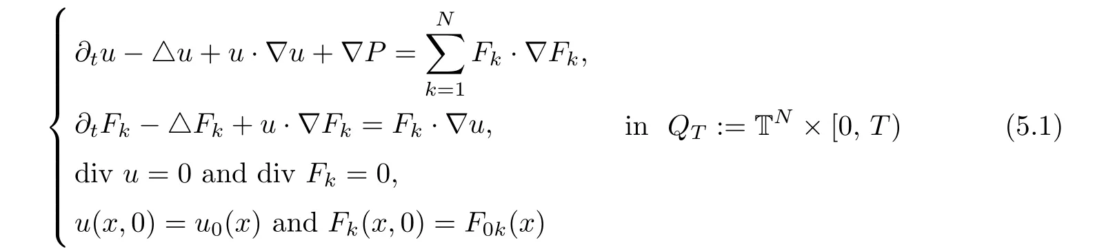
We consider the MHD equations in a periodic domain TNwith the periodic boundary condition as follows:
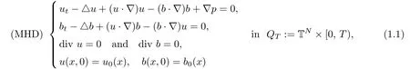
here u is the flow velocity vector,b is the magnetic vector and p is the total pressure.We consider the initial value problem of(1.1),which requires initial conditions

We assume that the initial data u0(x),b0(x)∈ L2(TN)hold the incompressibility,i.e.,∇·u0(x)=0 and∇·b0(x)=0,respectively.
For 3D MHD equations,it is well known that the global existence of weak solutions,local existence,and uniqueness of smooth solutions to the system(1.1)–(1.2)were established in[5,16].A lot of results for equations(1.1)are proved in view of partial regularity or or blow-up(or regularity)conditions and temporary decay(see e.g.[1–3,7,8,14,15,20,21,23,24,26]).
It is known that any weak solution becomes regular in QT,if the following scaling invariant conditions,so called Serrin type’s conditions(see e.g.[7])are satis fied

On the other hand,Shinbrot[17]showed the same conclusion if u∈Lp(0,T;Lq(TN)),where≤1 with q≥4 in case Navier-Stokes equations.It is interesting that the dimension N plays no part in the conditions imposed on u although it is hard to say which condition above is weaker.
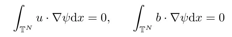
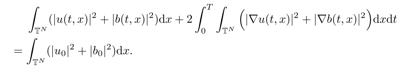
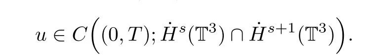
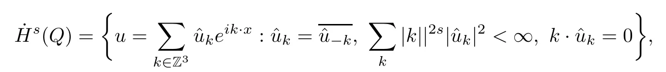
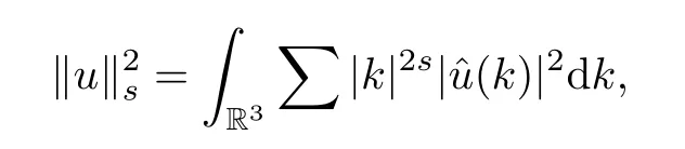
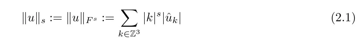
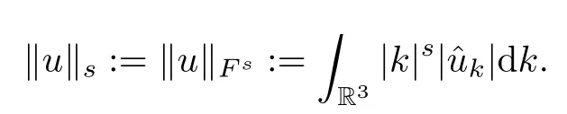
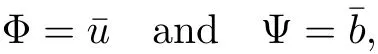
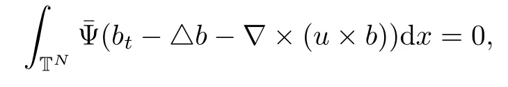
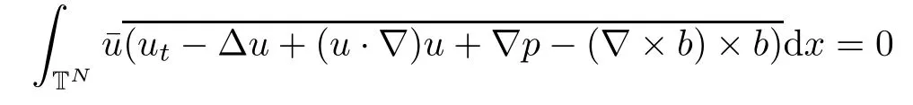
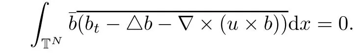
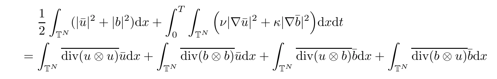
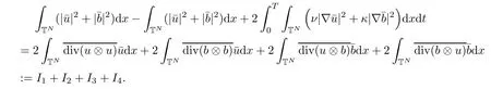
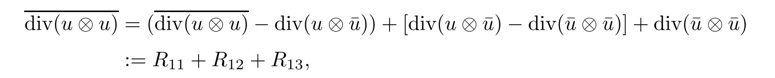
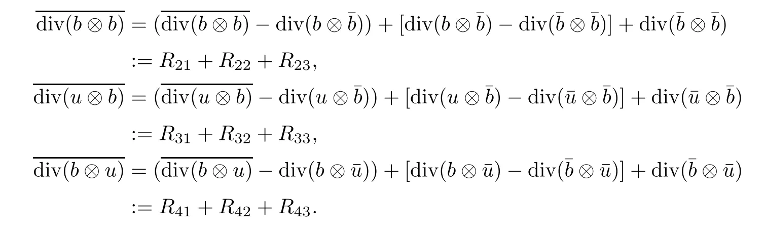
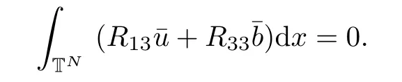
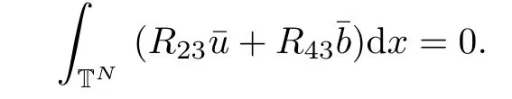
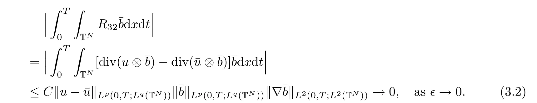
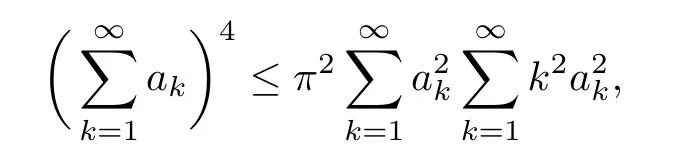
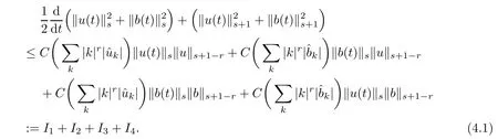
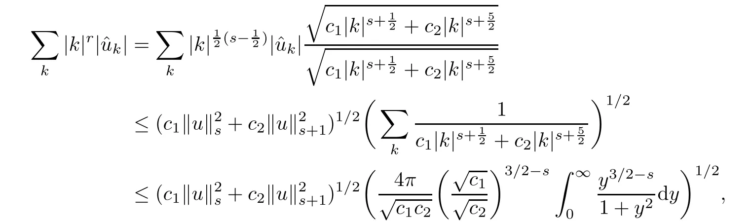
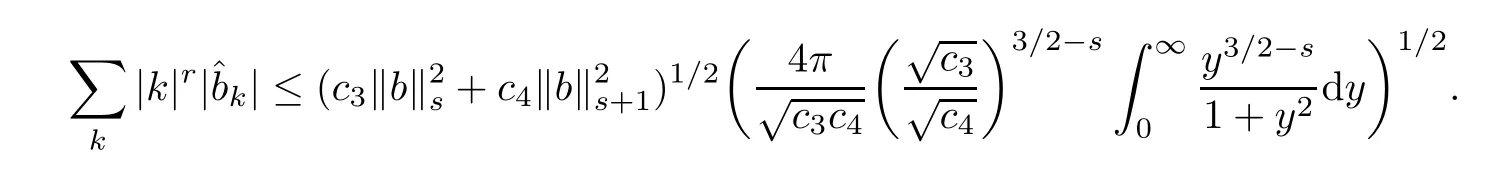
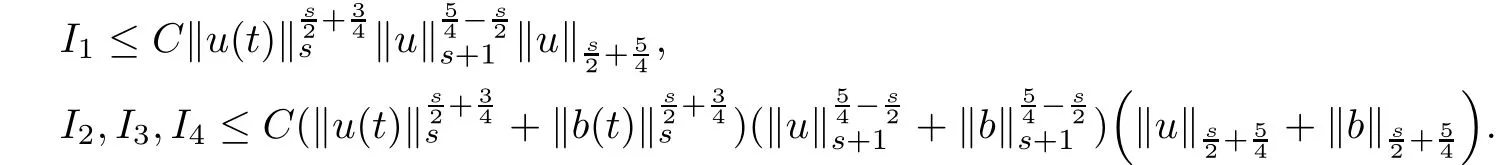
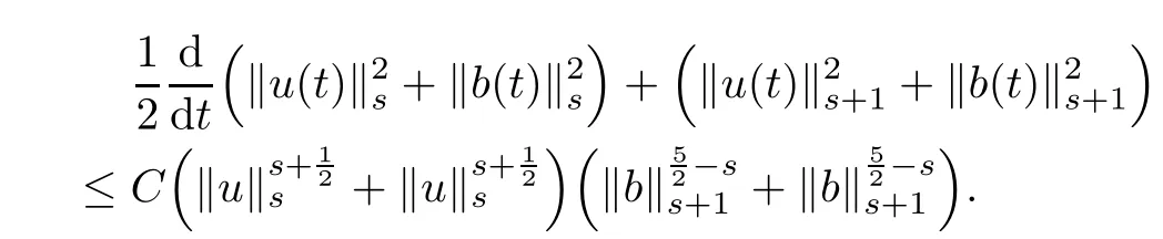
The purpose of this paper is twofold.First,we extend Shinbrot’s result to the 3D incompressible MHD equations(1.1)–(1.2).More speaking,it is shown that a weak solution of this system lying in a space Lq(0,T;Lp(TN)),where 2/p+2/q≤1 and q≥4,satis fies an energy equality rather than the usual energy inequality according to the argument in[25].Second,we give optimal lower bounds for the blow-up rate of the˙Hs-norm,1/2 Now,we recall first the de finition of a weak solution. De finition 1.1Let u0,b0∈L2(TN)with the divergence free condition.We say that(u,b)is a weak solution of the equations(1.1)–(1.2)if u and b satisfy the following (i) u ∈ L∞([0,T);L2(TN))∩L2([0,T);H1(TN)),b∈ L∞([0,T);L2(TN))∩L2([0,T);H1(TN)). (ii)(u,b)satis fies(1.1)in the sense of distribution,that is, The first result is to show the energy conservation for the weak solutions to the system(1.1)–(1.2)applying Yu’s argument[25](in the sense of Shinbrot’s sprit[17])based on Lemma 3.1 below. Theorem 1.2Let u,b∈L∞(0,T;L2(TN))∩L2(0,T;H1(TN))be a weak solution of the incompressible MHD equations in the sense of De finition 1.1.In additional,if u∈Lr(0,T;Ll(TN))for any,l≥4,then Moreover,the second result of this paper is to show the lower bounds for possible singular solutions to the system(1.1)–(1.2)in T3using the method in[4]based on Carlson’s inequality[11]. Theorem 1.3Let(u,b)be a solution to the incompressible 3D MHD equations(1.1)whose maximum interval of existence is(0,T),0 Then the following estimate holds Remark 1.4Theorem 1.2 and Theorem 1.3 also hold for R3because we don’t consider the boundary condition of a domain for our analysis. In this section,we collect notations and de finitions used throughout this paper.We also recall some lemmas,which are useful to our analysis.Let I=(0,T)be a finite time interval.For 1 ≤ q ≤ ∞,Wk,q(TN)indicates the usual Sobolev space with standard norm,i.e.,Wk,q(TN)={u ∈ Lq(TN):Dαu ∈ Lq(TN),0≤ |α|≤ k}.In case that q=2,we write Wk,q(TN)as Hk(TN).All generic constants will be denoted by C,which may vary from line to line. Let Q=[0,2π]3.We write Z3=Z3{0,0,0},let˙Hs(Q)be the subspace of the Sobolev space Hsconsisting of divergence-free,zero-average,periodic real functions In our estimates we will also use the L1-type norms of the Fourier transform, and We denote by Fsthe space of all those u for whichis finite. The goal of this section is to prove Theorem 1.2.To this end,we need to introduce a crucial lemma.The key lemma is as follows which was given in[13]. Lemma 3.1Let f∈W1,p(TN)and g∈Lq(TN)with 1≤p,q≤∞,and≤1. Then,we have for some C ≥ 0 independent of ǫ,f and g,r is determined by.In addition, as ǫ→ 0 if r< ∞,here ǫ>0 is a small enough number,η ∈(TN)be a standard molli fi er supported in B(0,1). The weak solutions u and b are uniformly bounded in L∞(0,T;L2(TN))∩L2(0,T;H1(TN)).Thus,it is possible to make use of Lemma 3.1 to handle convective terms involving u and b.With Lemma 3.1 in hand,we are ready to prove our main result.For this,we de fine a new function where f(t,x)=f∗ηε(x),ε>0 is a small enough number,η∈(TN)be a standard molli fi er supported in B(0,1). and which gives us and This yields and hence Note that Using the divergence free condition forand,we have Z And thus by the cancellation property for convection terms with the integration by parts,we also get Z Now we first assume that This restriction will be improved later.We can control the term related to R32in the following way Due to Lemma 3.1,we have and it converges to zero inas ǫ tends to zero.Thus,the convergence of R31gives us as ǫ→ 0.Thus,the convergences(3.2)and(3.3)imply In the same manner,we can easily check that The convergences for(3.4)and(3.5)imply the energy equality for any weak solutions with additional condition(3.1). Finally,it is to improve the restriction p≥4,q≥4.Using Gagliardo-Nirenberg inequality,u∈L∞(0,T;L2(TN))and u∈Lr(0,T;Ls(TN)),we get We recall Carlson’s inequality[11],which is key lemma to show Theorem 1.3. Lemma 4.1If a1,a2,···are real numbers,not all zero,then where the constant π2is sharp. Recall the estimate for the convection term given in[18,Lemma 3.1]. Lemma 4.2For any s≥0, Proof of Theorem 1.3First,for 0≤r≤1, Now,following the argument in[4],we pick r=(s−),and apply Lemma 4.1,to the first factor on the right hand side of(4.1),to obtain where we use the de finition ofgiven in(2.1)in first inequality and apply the interpolation technique employed by Hardy in his proof of Lemma 4.1 in last inequality(compare to[11]). And similarly,we have Using estimate(4.2)and Young’s inequality,we have By interpolation inequality,we get With(4.3)and the estimates I1–I4,inequality(4.1)becomes It is time to use Young’s inequality to get Finally,by integrating between T−t and T the previous estimate,inequality(1.3)follows.? Our arguments also allow to prove Theorems 1.2 and 1.3 for the incompressible viscoelastic equations with damping(see e.g.[9,12])as a way of approximating solutions of the viscoelastic model which describes an incompressible non-Newtonian fl uid,which the property of materials that exhibit both viscous and elastic characteristics when undergoing deformation(see[6,10,22]and references therein for physical background) with k=1,···,N,here u=u(x,t) ∈ TNrepresents the fl uid’s velocity,p=p(x,t) ∈ R represents the fl uid’s pressure,and F=F(x,t) ∈ RN× RNrepresents the local deformation tensor of the fl uid.We denote(∇ ·F)i=for a matrix F,in the(i,j)-th entries,i,j=1,2,···,N.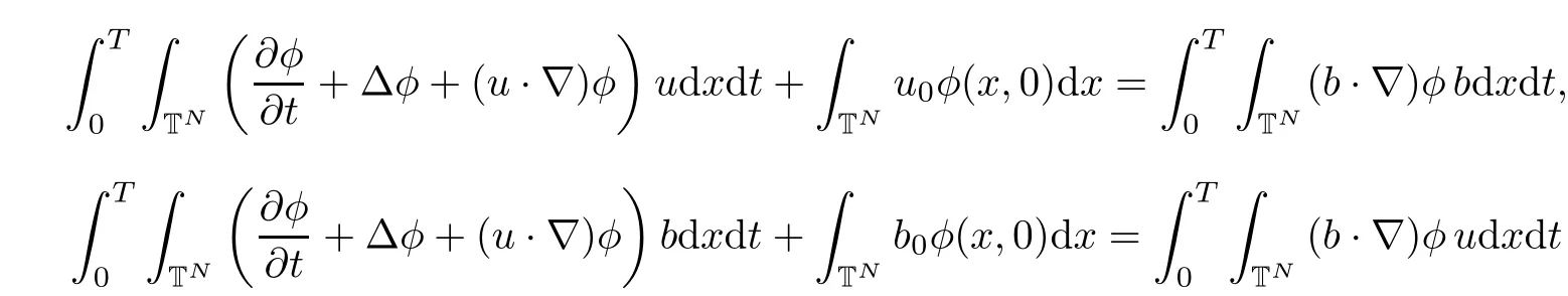

2 Preliminaries
3 Proof of Theorem 1.2


4 Proof of Theorem 1.3


5Remark
 Acta Mathematica Scientia(English Series)2020年1期