A High Order Formula to Approximate the Caputo Fractional Derivative

R. Mokhtari · F. Mostajeran

Abstract We present here a high-order numerical formula for approximating the Caputo fractional derivative of order α for 0 ＜α＜ 1. This new formula is on the basis of the third degree Lagrange interpolating polynomial and may be used as a powerful tool in solving some kinds of fractional ordinary/partial differential equations. In comparison with the previous formulae, the main superiority of the new formula is its order of accuracy which is 4-α, while the order of accuracy of the previous ones is less than 3. It must be pointed out that the proposed formula and other existing formulae have almost the same computational cost. The eff ectiveness and the applicability of the proposed formula are investigated by testing three distinct numerical examples. Moreover, an application of the new formula in solving some fractional partial differential equations is presented by constructing a f niite difference scheme. A PDE-based image denoising approach is proposed to demonstrate the performance of the proposed scheme.

Keywords Caputo fractional derivative · Fractional partial differential equation · Finite difference scheme

1 Introduction

Nowadays, to provide a better approach for describing complex phenomenon in nature,the fractional calculus has been developed in both theory and application. By entering the fractional derivative into the engineering and science problems, dozens of fractional problems such as the fractional diff usion equation, the fractional advection-diff usion equation,the fractional Fokker-Planck equation, the fractional cable equation and many other equations have appeared in recent years. Among various def initions of the fractional derivative, the Caputo fractional derivative is one of the most important and applicable tools in time-dependent problems. In fact in almost all of the time-fractional partial differential equations, the time-fractional derivative is usually considered in the sense of Caputo. A concise and somewhat complete literature survey can be found in [ 18].

Due to the complexity of computing of some special functions, such as the Fox H function and the hyperbolic geometry function [ 23], and the diffi culties of f inding exact solutions for most fractional problems, many researchers are working on extracting useful numerical algorithms. Some successful methods are the f inite difference method (FDM) [ 2, 6, 21], the f inite element method [ 24], the method of discontinuous Galerkin [ 8, 9, 26, 27], the meshless method [ 28], and the spectral approximation [ 19]; among them, the FDM is especially favored thanks to its simplicity in both calculation and analysis.

Obviously, a suitable numerical diff erentiation formula is necessary for numerically solving some fractional differential equations involving fractional derivatives. To the best of our knowledge, the Grünwald-Letnikov (GL) formula and the L1 formula are two more important numerical diff erentiation formulae for discretizing fractional derivatives. For the fractional derivative of order α , the accuracy of the GL formula is of order one [ 7, 23], while the L1 formula can achieve an improved accuracy of order 2-α [ 16]. In fact, the L1 formula is established by a piecewise linear interpolation approximation for the integrand function on each small interval.By applying a higher-order interpolant instead of the linear interpolant to improve the numerical accuracy, Cao et al. [ 5], Gao et al. [ 12], and Lv and Xu [ 20] proposed some (3-α)-order formulae for the α -order Caputo fractional derivative. A three-point L1 approximation of the Caputo derivative with order 3-α has been also presented in [ 11]. Recently, Cao et al. [ 4] have presented a high-order algorithm with convergence order 4-α for the Caputo derivative, in which the coeffi cients and truncation errors of the proposed scheme are not discussed in detail.Moreover, the proposed method was used to present a higher-order numerical scheme to solve a time fractional advection-diff usion equation and its stability analysis was discussed by using the Fourier method. We also independently introduce a 4-α order algorithm for the Caputo derivative with a slightly diff erent approach, where the implementation of the proposed scheme is distinctive, the weight coeffi cients are exactly examined, and the truncation error in our work is precisely inspected. For this purpose, three distinct numerical examples for testing the truncation error of the proposed formula and two diff erent numerical examples of the time-fractional partial differential equations with the Caputo fractional derivative are carried out.

The objective of this paper is to establish an explicit high-order numerical diff erentiation formula for the Caputo fractional derivative and apply it to some schemes for numerically solving some fractional differential equations. Here after presenting a brief discussion about previous fractional numerical diff erentiation formulae for Caputo fractional of order α , i.e., L1 and L1-2 [ 12], we introduce L1-2-3 formula which has a better numerical accuracy compared to the L1 and L1-2 formulae. After that, we use the new L1-2-3 formula in various examples and make a comparison between the new and older formulae. Then, we construct a f inite difference scheme for solving a time-fractional diff usion equation involving the Caputo derivative and provide some examples. Moreover, this new scheme is applied to the image denoising. Finally, we conclude the paper with a brief conclusion.

2 New Formula, Construction and Properties

In this section, to fully understand the proposed process, after representing both the L1 formula and the L1-2 formula, we give a new process of deriving the fractional numerical differentiation formula called L1-2-3. For this purpose, we denote Δt as the temporal step length and for the integer k≥0 , we set tk=kΔt , tk+1∕2=(tk+1+tk)∕2 , and

Denoting linear Lagrange interpolant of f on each small interval [tj-1,tj](1≤j≤k) as Π1,jf , we get

which follows from the linear interpolation theory that

In a similar way, by constructing the second-degree Lagrange interpolating polynomial Π2,jf of f using three points (tj-2,f(tj-2)),(tj-1,f(tj-1)) , and (tj,f(tj)) and taking a constraint of the result onto small interval [tj-1,tj](2≤j≤k) , we have

and

For j≥3 , constructing the third degree Lagrange interpolating polynomial Π3,jf of f using four points (tj-n,f(tj-n)),n=3,2,1,0 and taking a constraint of the result onto the small interval [tj-1,tj](2≤j≤k) , we get

and immediately

where Φj(t)=3t2-2t(tj-2+tj-1+tj)+tjtj-1+tjtj-2+tj-2tj-1. Moreover, we know that

For further details about Lagrange interpolants, we refer to [ 3]. Letting f∈C1[0,tk] ,the Caputo fractional derivative of order α is def ined as [ 19]

In this paper, we assume that 0＜α＜1 . In ( 1), we use Π1,jf to approximate f on the f irst small interval [t0,t1] , Π2,jf to approximate f on the second small interval [t1,t2] and for j≥3 ,Π3,jf to approximate f on the interval [tj-1,tj] . Noticing

where

we can obtain an improved numerical approximation of the Caputo fractional derivative of order α for function f in the following form:

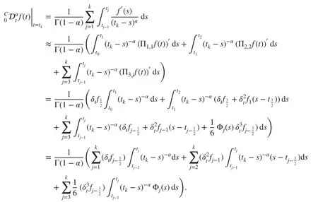
Lemma 2.1For any α , we have

ProofThe only root of Φjin [tj-1,tj] is[tj-1,tj] . Moreover, Φjis an increasing function on , and (tk-s)-αis a continuous, positive and increasing function of s on [tj-1,tj] . Using the weighted mean value theorem for integrals [ 3], we have

(a) there is c1∈[tj-1,] such that

(b) there is c2∈[,tj] such that

Therefore,

Again, using the weighted mean value theorem for integrals, we can write

(a) there is c1∈[tj-1,] such that

(b) there is c2∈[,tj] such that

where g(s)=(tk-s-Δt)-α-(tk-s)-αwhich is an increasing function of s on [tj-1,tj]since g′(s)=α((tk-s-Δt)-(α+1)-(tk-s)-(α+1))＞0 . Therefore, Ag(c1)＜Ag(c2) , and it means that

Then,

Knowing Φj(s)=Φj(s+Δt),s∈[tj-1,tj] , we have

Therefore, ( 5) holds, and so the proof is complete.

The new, improved fractional numerical diff erentiation formula ( 4) can be rewritten as

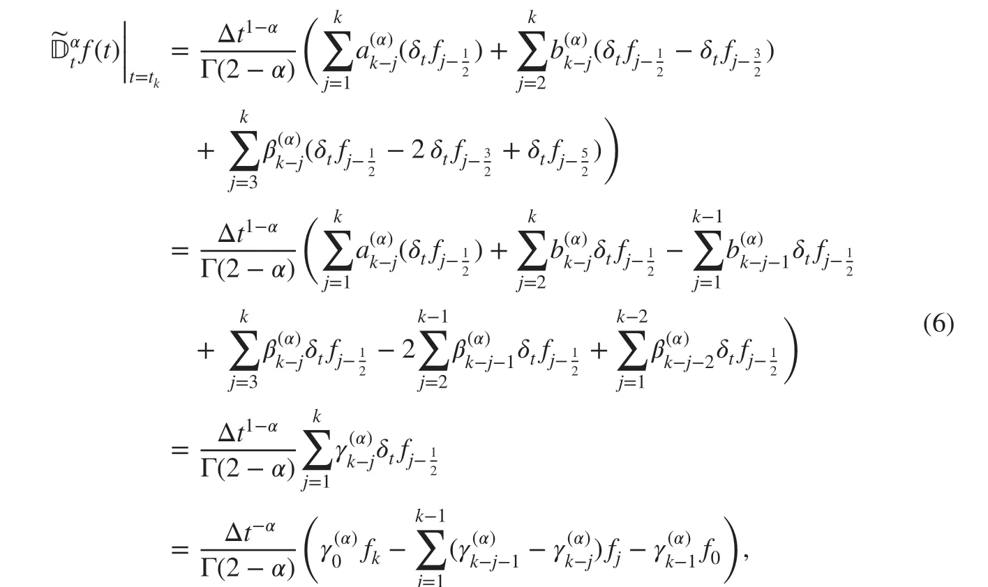
For k=1, ( 4) is the same as ( 2); for k=2 , ( 4) is the same as ( 3); for k=3,

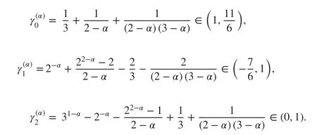
Lemma 2.2For any α and(0≤j≤k-1,k≥4) def ined in ( 7), we have

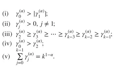
ProofFor any α and k≥4 , noticingin ( 7), we have

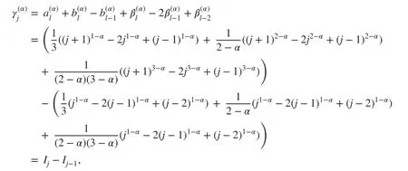
where

For x≥1 , we have h′(x)＞0,h′′(x)＞0,h′′′(x)＞0 , and h(4)(x)＜0 . Therefore,

where j-2＜ζj＜j+1 and j-2＜σj＜j+2 . That is to say that

In addition,

is continuous for all α∈[0,1] , then it attains its maximum and minimum values on [0, 1].

Because the minimum of this function on [0, 1] is zero,, soSimilarly,

is continuous for all α∈[0,1] , then due to attaining its minimum values on [0, 1], which is zero,thenMoreover,

is continuous for all α∈[0,1] . Because p′(α)＜0 on [0, 1], this function is decreasing on[0, 1], and then 0=p(1)＜p(α) for all α∈(0,1) ; thus,＞0 . In a similar way,

is continuous, thus for all α∈[0,1] . Because q′(α)＜0 on [0, 1], 0=q(1)＜q(α)for all α∈(0,1) ,. That is to say, (ii) and (iii) hold. Due to the fact thatis positive, continuous, and increasing on (0, 1), we haveso (iv) holds. The validity of (v) can be directly derived from the def niition( 7) of. The proof is completed.

The truncation errors of the new L1-2-3 formula ( 6) are illustrated in the following theorem.

Theorem 2.1Suppose f∈C4[0,tk]. For any α ,is def ined in ( 6). DenoteThen, we have

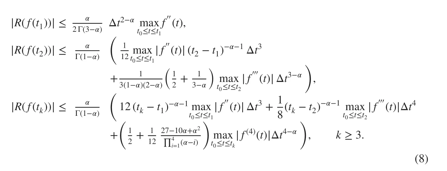
ProofFor k=1, ( 6) is just the L1 formula, and we have

where η1∈(t0,t1) . For k=2, ( 6) is just the L1-2 formula, and we have

where

and

where η2∈(t1,t2) . For k≥3 , we get

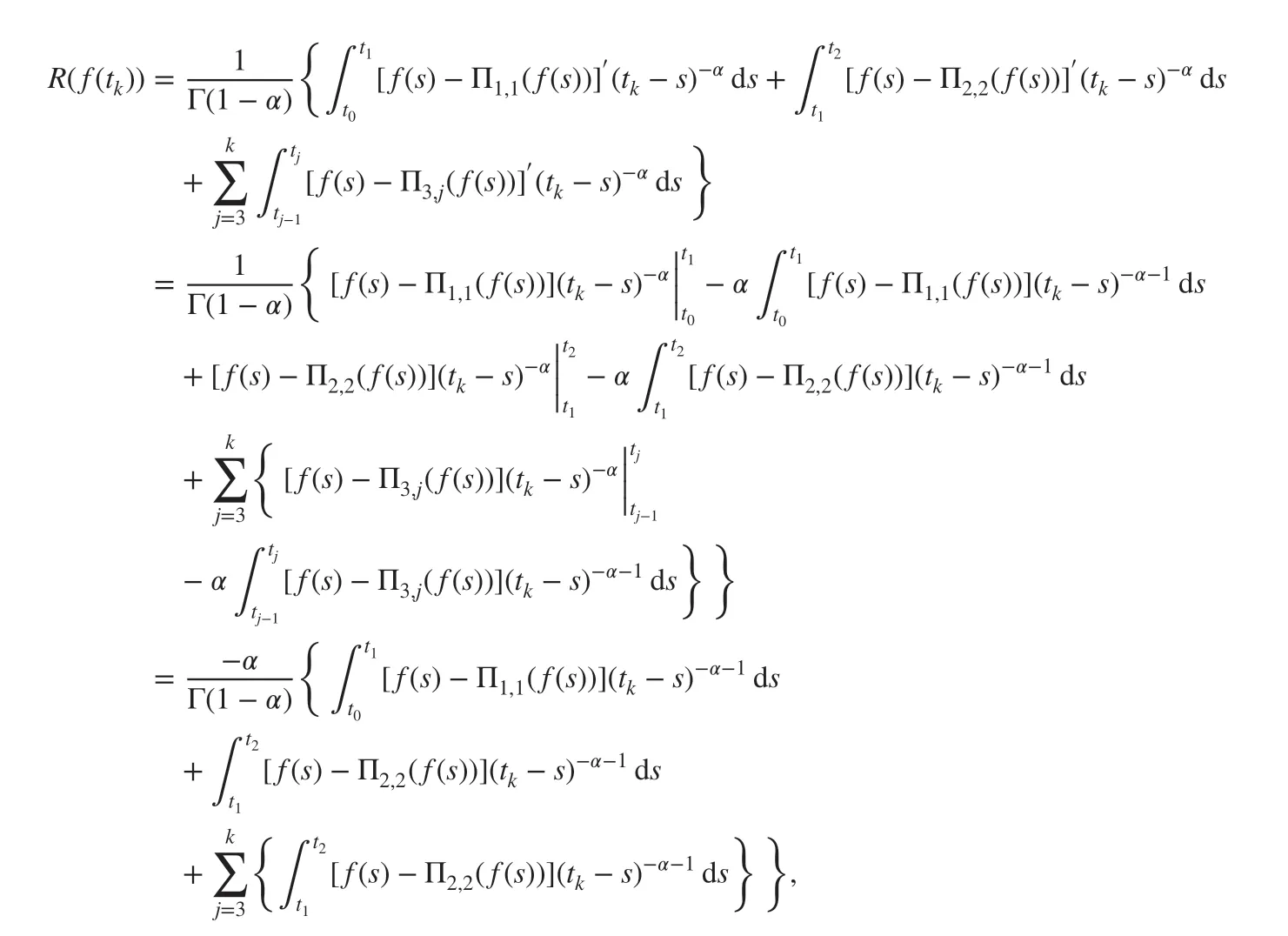
where

is used. Moreover,

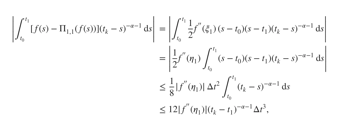
where η1∈(t0,t1),

where η2∈(t1,t2) , and

where ηj∈(tj-3,tj),3≤j≤k-1 , η∈(t0,tk-1) . In addition,

where ηk∈(tk-3,tk) . Hence, ( 8) holds.

3 Numerical Examples

To verify our constructed numerical formula for the Caputo fractional derivative and show that L1-2-3 formula ( 6) can act better than the L1 and L1-2 formulae, we test the following three numerical examples. Although the f irst two examples ( f(t)=t4+rand f(t)=t3)are polynomial-based examples with zero initial values, the convergence order of them is diff erent. In addition, the third one ( f(t)=exp(2t) ) is a non-polynomial example with nonzero initial value and its exact solution does not have a closed form. Actually, we aim to present these three examples to show that the convergence order of the formula depends on the function f. In fact, the convergence order of the following three examples are, respectively, 4-α , 4 and 3.

For 0≤k≤N, denote

and assume that tN=T=1.

Example 1Let f(t)=t4+r, where 0≤r＜1 . We compute the α-order Caputo fractional derivative of f( T) numerically. The exact solution is given by

We use three methods presented in Sect. 2, and list the computational errors and numerical convergence orders for diff erent parameters α=0.9,0.5,0.1 and diff erent temporal step sizes in Table 1. Noticing Table 1, we f ind that the computed errors by the L1-2-3 formula ( 6)are obviously much smaller than that by the L1-2 and L1 formulae ( 3) and ( 2), and the attainable convergence order of the L1-2-3 formula ( 6) is 4-α , which is also higher than the convergence order of 3-α and 2-α for the L1-2 and L1 formulae ( 3) and ( 2). From the above test example, we can draw the conclusion that the computational effi ciency and numerical accuracy of the new formula ( 6) are superior to that of the L1-2 formula ( 3) and L1 formula( 2), and the convergence order of ( 6) reaches 4-α if N≠1 and N is relatively large.

Example 2Consider f(t)=t3. We compute the α-order Caputo fractional derivative of f( T) numerically. The exact solution is given by

Taking the same varying temporal step sizes and parameters α as in Example 1, we use formulae ( 2), ( 3), and ( 6), and list the computational errors and numerical convergence orders in Table 2. According to ( 8), for f(t)=t3, we have

which shows that the convergence order of ( 6) for this example reaches 4 since(tk-t1)-α-1=O(1) and (tk-t2)-α-1=O(1) . The results of Table 2 conf irm this fact.

Example 3Suppose f(t)=exp(2t) . We compute the α-order Caputo fractional derivative of f( T) numerically. The exact solution is given [ 10] by

where Eμ,ν(z) is the Mittag-Leffl er function with two parameters def ined by

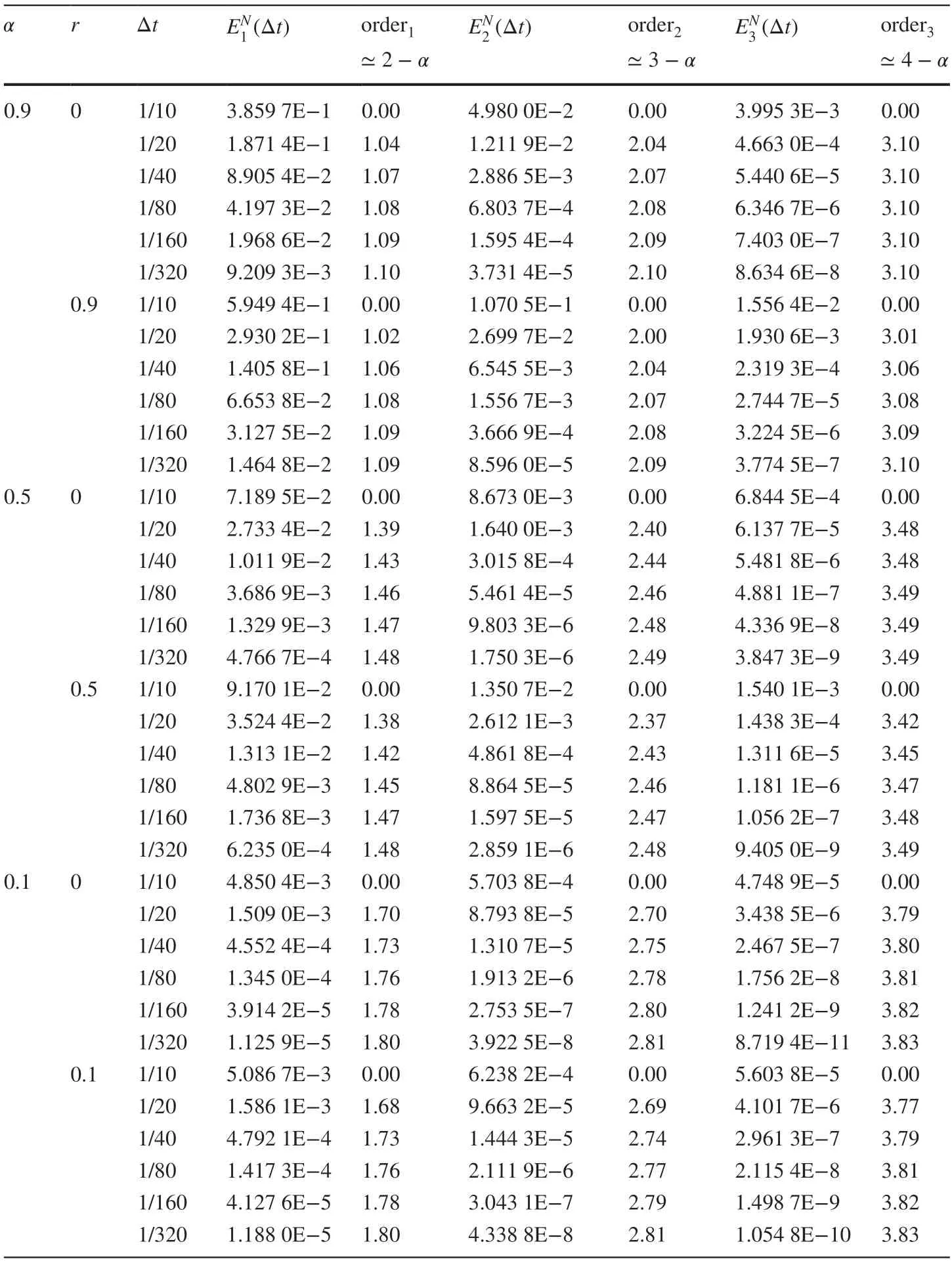
Table 1 (Example 1) Computational errors and convergence orders

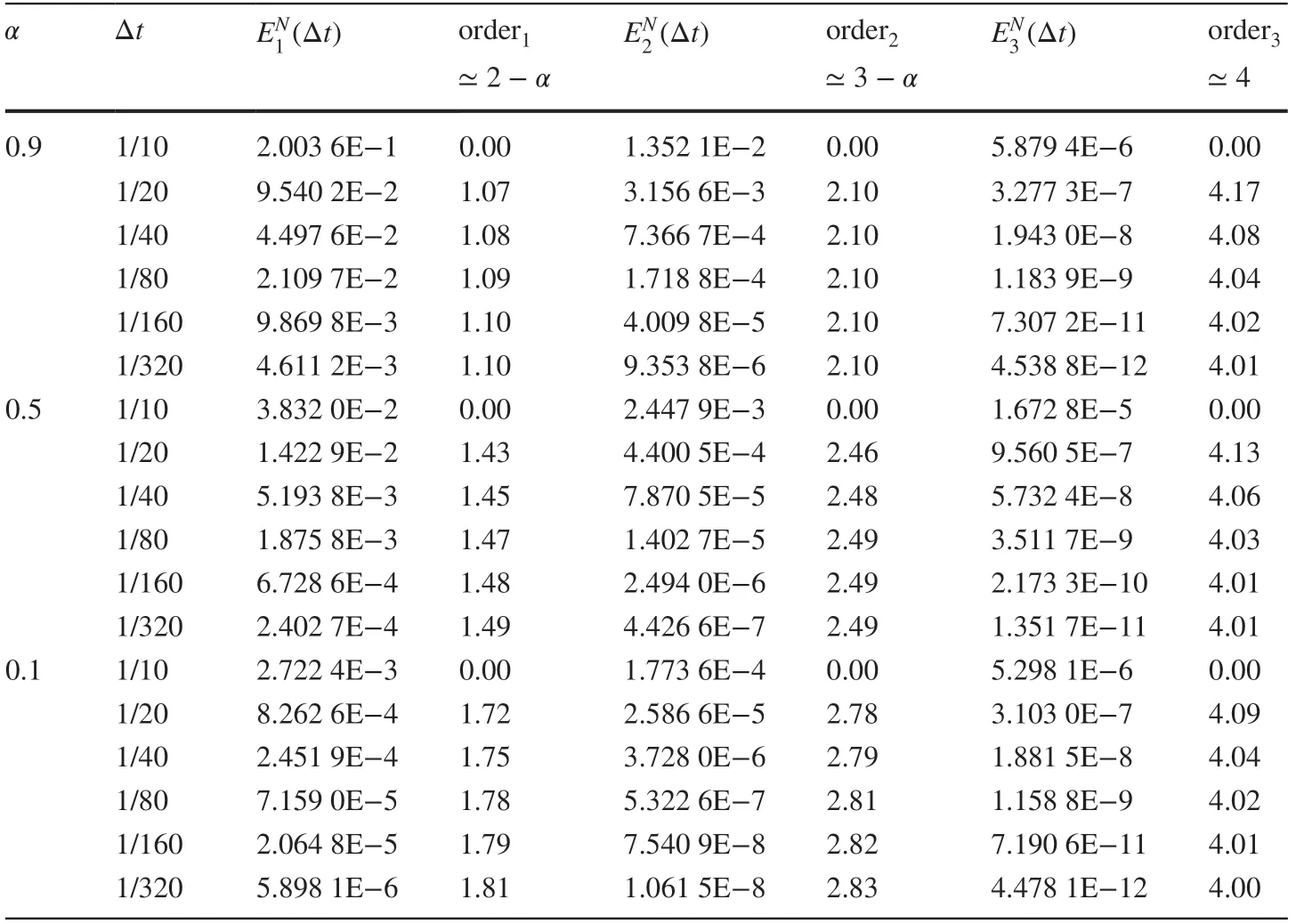
Table 2 (Example 2) Computational errors and convergence orders

Due to the lack of closed form for the exact solution of this problem, the Mittag-Leffl er function Eμ,ν(z) which depends on the precise values of the parameters μ and ν and the argument z has been numerically computed. Table 3 is reported to make a comparison with [ 4].According to the results of Table 3, numerical convergence order of formula ( 6) reaches 3.Also, being determined by ( 8), for f(t)=exp(2t) , we have

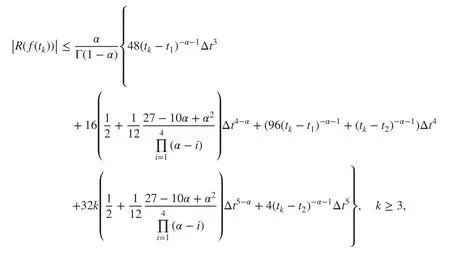
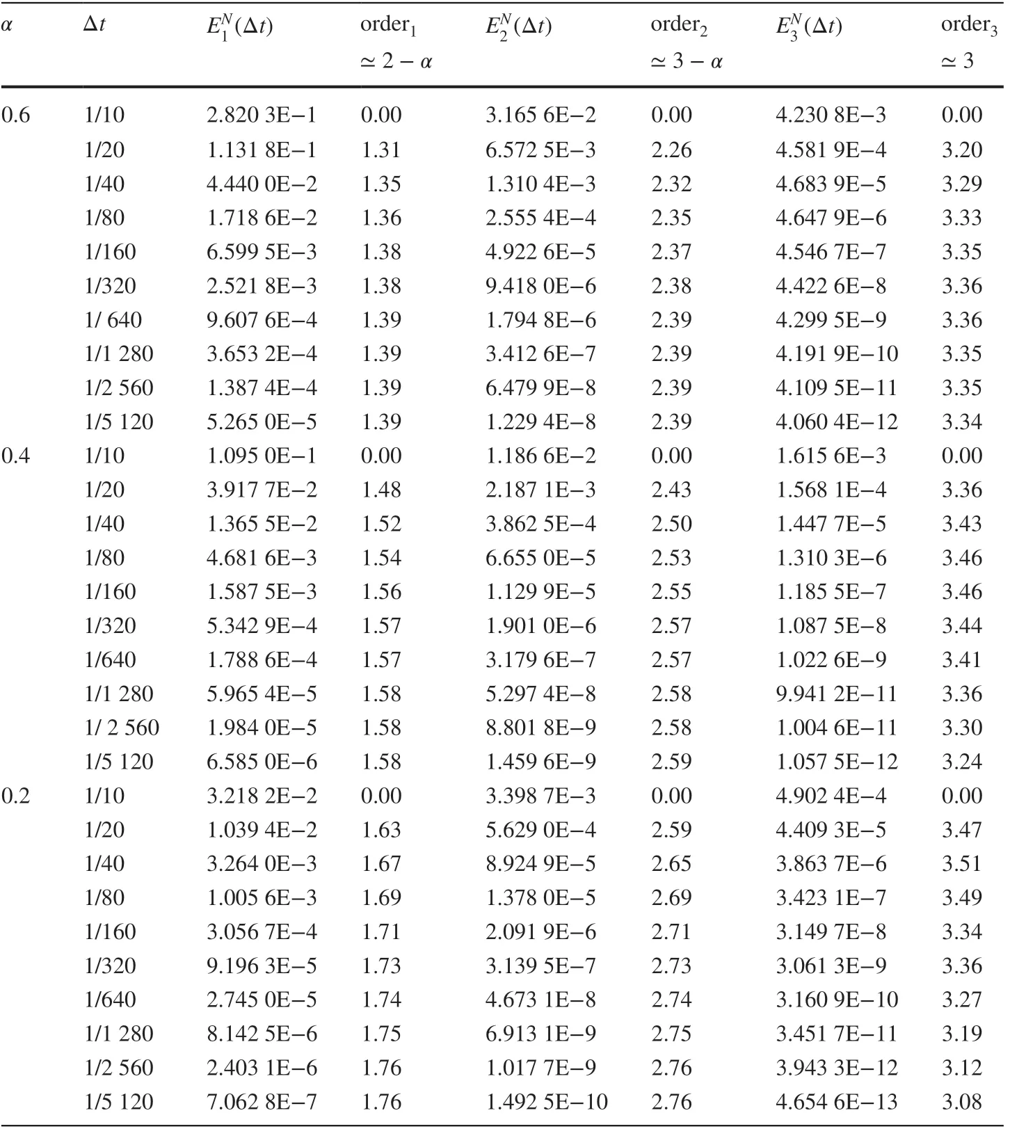
Table 3 (Example 3) Computational errors and convergence orders

which shows that the convergence order of ( 6) for this example must be 3, since(tk-t1)-α-1=O(1) and (tk-t2)-α-1=O(1) . Since truncation error of the new L1-2-3 formula has not been obtained correctly in [ 4], the authors claimed and showed that the convergence order of ( 6) for this example is 4-α, which is not correct. Specif ically, for α=0.8 , when the temporal step size has decreased to 1/5 120, the convergence order has increased to 3.196 2, which seems to reach 4-α . Nevertheless, for this value of α , the convergence order will steadily decrease and reach 3 when Δt decreases to less than 1/40 960. For these three numerical tests, Fig. 1 shows that the computational error curves with α=0.5 and N=20 using three diff erent formulae, the L1 formula ( 2), L1-2 formula ( 3),and L1-2-3 formula ( 6). According to Fig. 1, it is clearly obvious that the computational results by ( 6) are better than the ones by ( 2) and ( 3).

Fig. 1 The error curves of absolute errors with α=0.5,N=20

3.1 Time-Fractional Partial differential Equations

We carry out in this section a series of numerical examples of time-fractional partial differential equations with the Caputo fractional derivatives and present some results to conf irm our theoretical statements. The main purpose is to check the convergence behavior of the numerical solution with respect to the time step Δt . Consider the time-fractional diff usion equation of the form

subject to the following boundary and initial conditions:

where α is the order of the Caputo fractional derivative, T＞0 , and f,φ,φ , and u0are given functions. Introducing a f inite difference approximation to discretize the time-fractional derivative, let ΩΔt={tk|tk=kΔt,k=0,1,…,N}, where Δt=T∕N is the time step size.By using ( 6), Eq. ( 9) is converted to

where μ=(Δt)αΓ(2-α) , and according to Theorem 2.1 for k≥3,

Let uk=uk(x) be the numerical approximation to u(x,tk) , and fk=f(x,tk) . Then,Eq. ( 11) can be discretized as the following scheme:

To discretize ( 11) in space, let ΩΔx={xi|xi=iΔx,i=0,1,…,M} , where Δx=1∕M is the space step size. Suppose u={|0≤i≤M,0≤k≤N} is a grid function on ΩΔx×ΩΔt, and introduce, whereis the f irst-order difference quotient of u on the points ( xi,tk) and ( xi-1,tk) , andwhereis the second-order difference quotient of u on the points (xi-1,tk) , (xi,tk) and(xi+1,tk) . The f inite difference scheme which we consider for ( 9) and ( 10) is as follows:

Remark 3.1The truncation error of ( 13) is

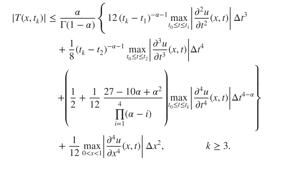
The corresponding difference schemes using the L1-2 formula [ 12] and L1 formula [ 25]for the Caputo derivative are, respectively,

where j=1,2,3 . To test the effi ciency of the difference scheme ( 13), two numerical examples, which have diff erent nature (in particular, in the time-dependent part of the solution and therefore in the initial condition which aff ect the convergence order of the formula) are examined.

Example 4In ( 9) and ( 10), takeu0(x)=0 . The exact solution is u(x,t)=ext4+α. and

Table 4 (Example 4) Numerical results of f inite difference schemes with Δx=1∕20000

Fig. 2 The absolute errors and CPU time versus cell number N with α=0.1,Δx=1∕1000

In Table 4, the numerical results using difference schemes ( 15), ( 14), and ( 13) for T=1 are computed. Due to verifying the temporal numerical accuracy, a f ixed and suffi cient small spatial step size Δx (Δx=1∕20000) is chosen. Noticing Table 4, we f ind that the computational errors of the difference scheme ( 13) are smaller, and its numerical accuracy is superior to the results of 3-α order of accuracy of ( 14) and 2-α order of accuracy of ( 15) in time.Moreover, for T=1 and α=0.1 with Δx=1∕1000 and diff erent temporal step sizes, the cell numbers N and the CPU time (on the same machine equipped with Intel 2.4-GHz Intel Core processor, Matlab software) are recorded when the absolute errors of three schemes are on the same orders. According to Fig. 2 showing the relationship between N, absolute errors, and CPU time for three schemes, the cell number N would be much smaller for the scheme ( 13)than for the schemes ( 14) and ( 15). It is clearly obvious that the larger temporal step size can be used for the scheme ( 13) than for the other two schemes. In addition, Fig. 2 shows that for the same absolute errors, the CPU time is much shorter by using the scheme ( 13) than that by using the schemes ( 14) and ( 15). To reach absolute error less than 5E-8 when T=1,α=0.1 ,and Δ x=1∕1000 , we must computeandwhich are, respectively, the solution of scheme ( 13), ( 14), and ( 15). For obtaining, we need three arrays with dimension 80×1 , 7 9×1 , and 7 8×1, respectively, to computeand; for obtaining, we need two arrays with dimension 4 10×1 and 4 09×1, respectively, to computeand;and for obtainingwe need one array with dimension 6 800×1 to compute. Therefore, we can draw a conclusion that less memory for computing(obtained by L1-2-3) is required.

Example 5In ( 9) and ( 10), take T=1,f(x,t)=ex[2t1-αE1,2-α(2t)-e2t],φ(t)=e2t,φ(t)=e1+2t, and u0(x)=ex. The exact solution is u(x,t)=ex+2t.

The computational results listed in Table 5 state the advantages of the difference scheme ( 13) over ( 14) and ( 15). Noticing this table, we f ind that the computational effi ciency and numerical accuracy of the difference scheme ( 13) are better; moreover, its convergence order of ( 13) is superior.

To investigate the numerical stability of scheme ( 13), we only follow up some tests and report corresponding results in Tables 6 and 7. Results imply that even by setting large time and space step sizes, satisfactory results may be produced and there is no track of the instability. So it seems that the method is unconditionaly stable, but proving this fact needs a rigorous and strict theoretical analysis which we leave it to future works.

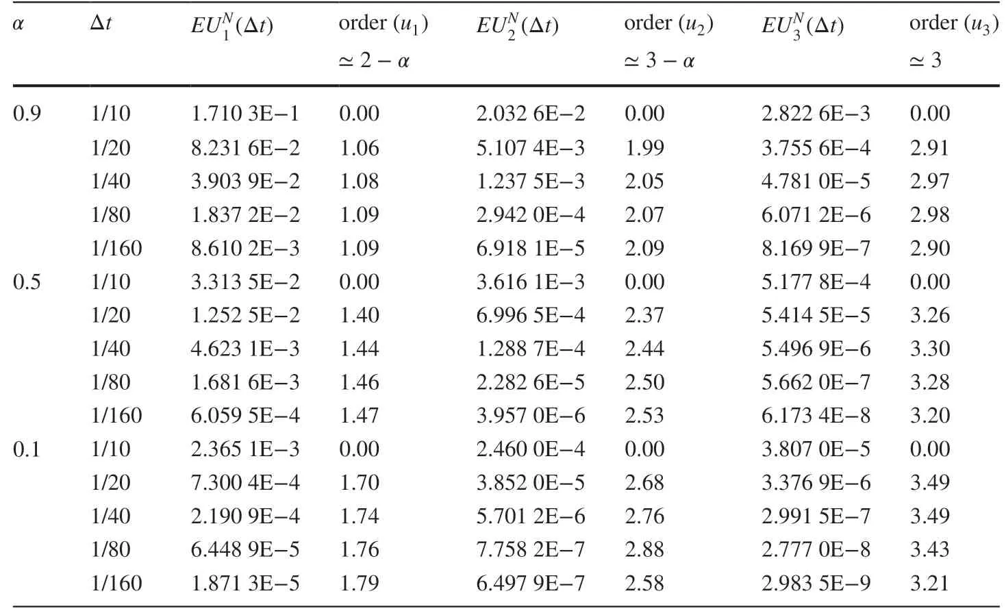
Table 5 (Example 5) Numerical results of f inite difference schemes with Δx=1∕20000

Table 6 Numerical stability analysis of f inite difference scheme ( 13) (Part I)

3.2 PDE-Based Image Denoising

Image noise removal constitutes a very important process; the most common noise results from the image acquisition system can be modeled as Gaussian random noise in most cases. Gaussian noise represents statistical noise having the probability density function equal to that of the normal distribution. Numerous image denoising models have been introduced in the past few decades. Although the conventional f ilters such as averaging f ilter, median f ilter, and the 2D Gaussian f ilter are effi cient in smoothing the noise, they have the disadvantage of blurring image edges [ 13, 15]. PDE-based methods for image processing (denoising, restorations, inpainting, segmentation, etc.) have been largely studied in the literature [ 1] due to their remarkable advantages in both theory and computation. To preserve the image structures when removing the noise, Perona and Malik (PM) [ 22] proposed a nonlinear equation which replaced isotropic diff usion expressed through a linear heat equation with an anisotropic diff usion. While the backward diff usion of the PM equation results in enhancing the edges, it is an ill-posed process in the sense that it is very sensitive to perturbations in the initial noisy data. Since the work of Perona and Malik, a large number of nonlinear PDE-based anisotropic diff usion models have been proposed [ 14, 17].

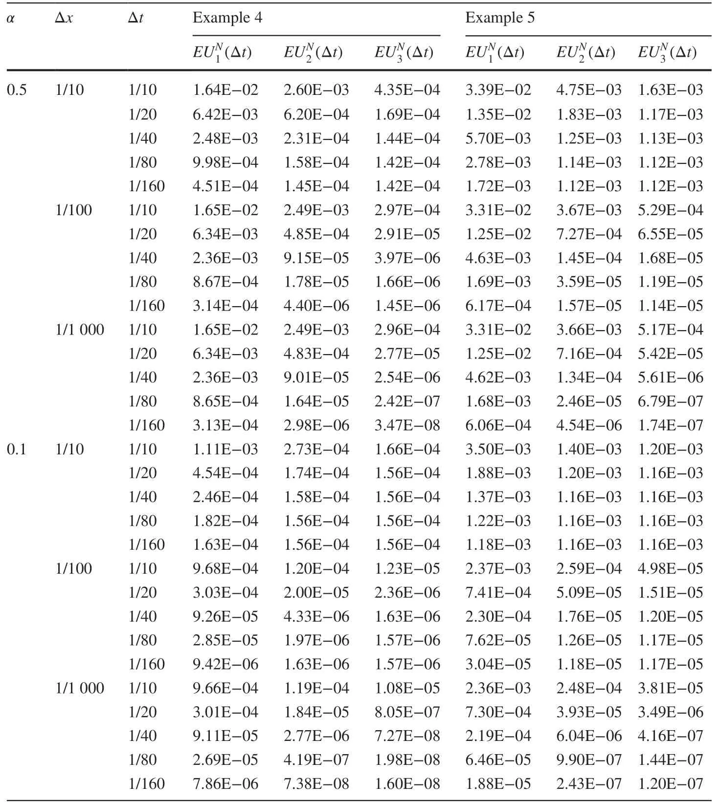
Table 7 Numerical stability analysis of f inite difference scheme ( 13) (Part II)

In this section, to conf irm the ability of the new L1-2-3 formula to solve fractional differential equations in two dimension and illustrate the applications of it in image denoising,the fractional-order PDE has been applied to the image processing and computer vision.We proposed a fractional-order equation for image denoising as where Δ denotes the Laplacian operator, Ω⊂ℝ2represents the image domain, andstands for the Caputo fractional time derivative of order α . Assume that an image has (Mx+2)×(My+2) pixels, and≃u(i,j,tk) for i=0,1,…,Mx+1 and j=0,1,…,My+1 . The following explicit f inite difference scheme by using L1-2-3 formula ( 6) to approximate the time-fractional derivative and the second-order central difference quotient has been considered for ( 16):to treat the spatial derivative term. Here μ=(Δt)αΓ(2-α) ,is an image aff ected by a noise, and the boundary conditions are zero. Similarly, the following explicit f inite difference scheme by using L1-2 formula to approximate the time-fractional derivative term has been considered for ( 16)

where U is an initial image and u is a restored version. Due to the purpose of the paper,developing a fractional numerical diff erentiation formula called the L1-2-3 formula to approximate the Caputo fractional derivative of order α , the denoising performance of our method has not been compared with performances of other noise removal techniques. The images shown in Fig. 3 a represents the original [512×512] image of Baboon; (b) represents the degraded image by Gaussian noise characterized by parameters 0.1 (mean) and 0.01 (variance); (c, e) represent the image denoising result produced by the L1-2 model( 18) with α=0.4,N=25 and α=0.5,N=8 ; (d, f) represent the image denoising result produced by the L1-2-3 model ( 17) with α=0.4,N=25 and α=0.5,N=8 . Another two image denoising method comparison examples are displayed in Figs. 4 and 5. The same noise removal approaches are applied on the standard Lena and Peppers images corrupted by the same amount of Gaussian noise, their results being represented in Figs. 4 c-f and 5 c-f. According to Table 8, the values of PSNR for noise reduction approaches corresponding to Figs. 3- 5, the L1-2-3 model ( 17) can smooth the noise better than the L1-2 model ( 18).

4 Conclusion

In this work, a new fractional numerical diff erentiation formula called the L1-2-3 formula, obtained by constructing a third degree Lagrange interpolation function for the integrand f, is established to approximate the Caputo fractional derivative of order α .After providing some analysis for the coeffi cient features and truncation errors of the L1-2-3 formula and considering two test examples which are conducted to eff ectively conf irm its computational validity and numerical accuracy, we apply it in solving some time-fractional sub-diff usion equations on a bounded spatial domain. To illustrate the effi ciency and advantages of the proposed scheme, we use it for smoothing the noise of some digital images. Some numerical tests imply that the scheme is unconditional stable.Providing a rigorous theoretical stability analysis of the proposed scheme can be considered as a future work.

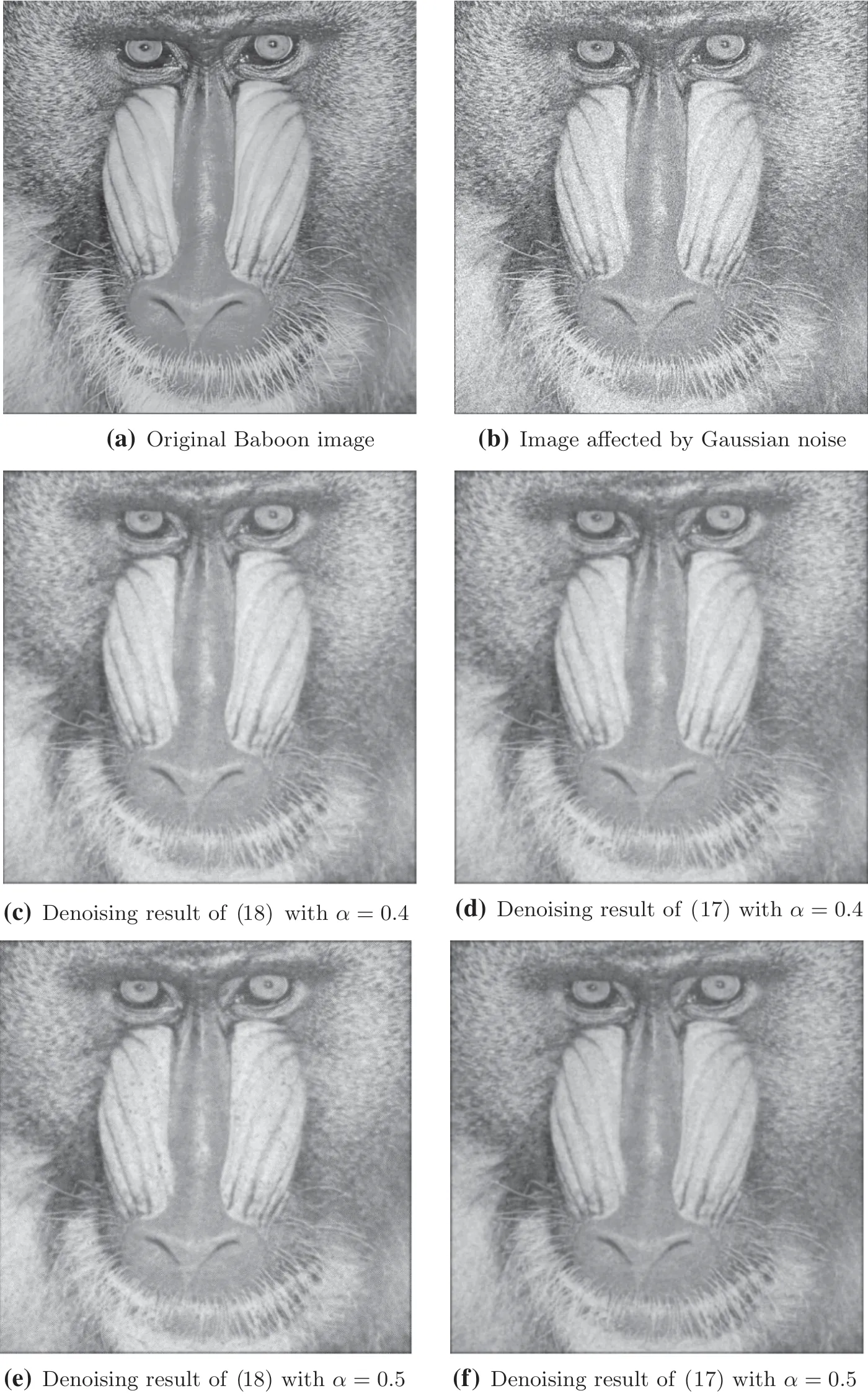
Fig. 3 Gaussian noise removal results produced by the L1-2 model ( 18) and the L1-2-3 model ( 17)

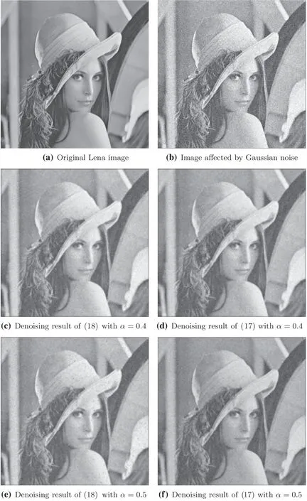
Fig. 4 Gaussian noise removal results produced by the L1-2 model ( 18) and the L1-2-3 model ( 17)

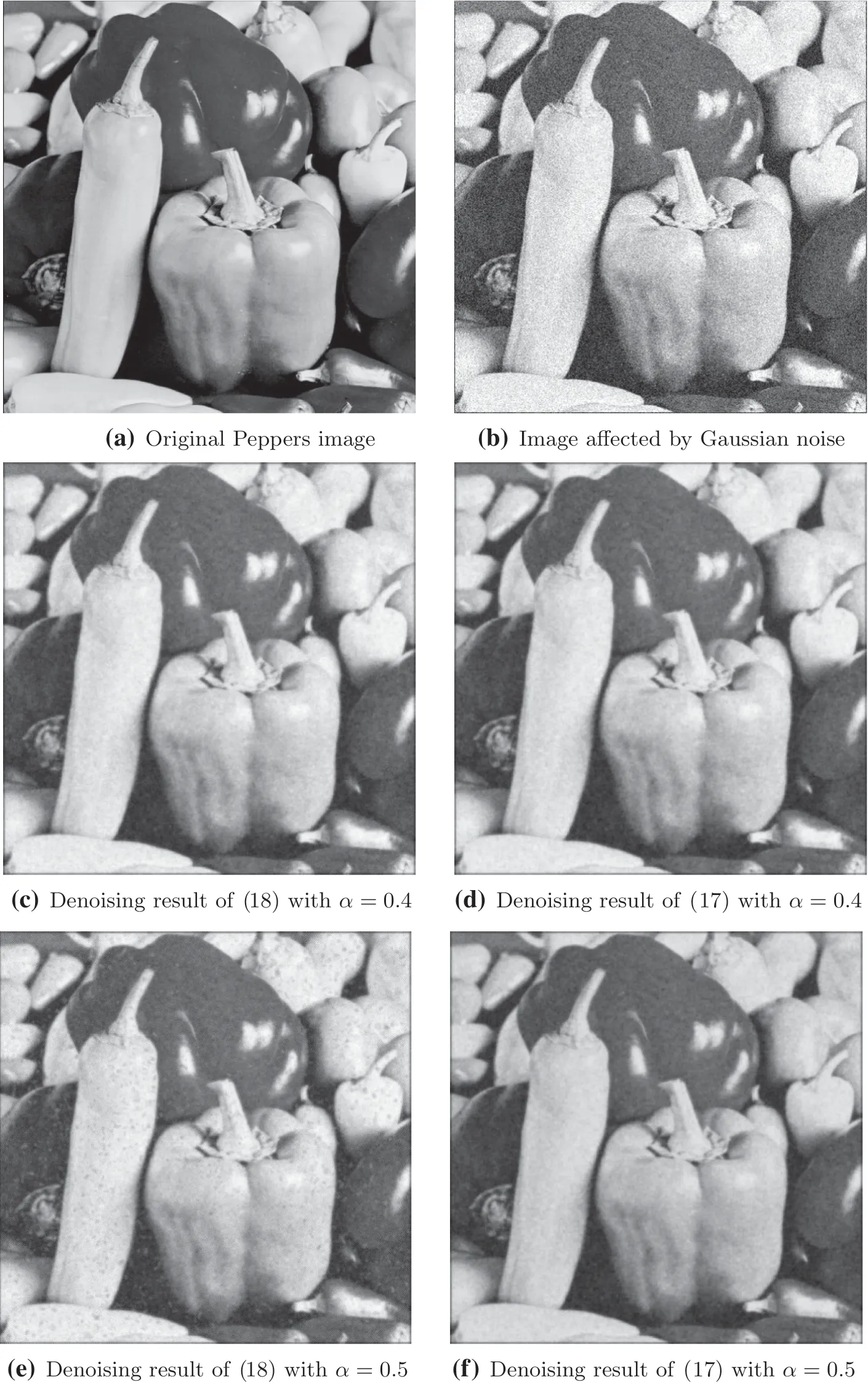
Fig. 5 Gaussian noise removal results produced by the L1-2 model ( 18) and the L1-2-3 model ( 17)

Table 8 Values of PSNR for noise reduction approaches

In summary, in comparison with the previous methods such as the L1-2 and L1 formulae, the convergence order of the L1-2-3 formula is higher and its computational effi ciency and numerical accuracy are superior. Moreover, this new formula can be used for both numerically solving other various fractional differential equations that involve the Caputo time-fractional derivatives and smoothing the noise. Experiments show improved performances in these areas.