Traffic prediction using a self-adjusted evolutionary neural network

Shiva Rahimipour· Rayehe Moeinfar · S. Mehdi Hashemi

Abstract Short-term prediction of traffic flow is one of the most essential elements of all proactive traffic control systems.The aim of this paper is to provide a model based on neural networks (NNs) for multi-step-ahead traffic prediction. NNs’ dependency on parameter setting is the major challenge in using them as a predictor.Given the fact that the best combination of NN parameters results in the minimum error of predicted output, the main problem is NN optimization.So,it is viable to set the best combination of the parameters according to a specific traffic behavior.On the other hand, an automatic method-which is applicable in general cases-is strongly desired to set appropriate parameters for neural networks.This paper defines a self-adjusted NN using the non-dominated sorting genetic algorithm II (NSGA-II) as a multi-objective optimizer for short-term prediction. NSGA-II is used to optimize the number of neurons in the first and second layers of the NN,learning ratio and slope of the activation function. This model addresses the challenge of optimizing a multi-output NN in a self-adjusted way. Performance of the developed network is evaluated by application to both univariate and multivariate traffic flow data from an urban highway.Results are analyzed based on the performance measures,showing that the genetic algorithm tunes the NN as well without any manually pre-adjustment. The achieved prediction accuracy is calculated with multiple measures such as the root mean square error (RMSE), and the RMSE value is 10 and 12 in the best configuration of the proposed model for single and multi-step-ahead traffic flow prediction, respectively.

Keywords Traffic prediction · Neural networks · Genetic algorithm · Self-adjusted framework

1 Introduction

Intelligent transportation systems (ITSs) are expected to alleviate traffic problems around the world. Short-term traffic prediction is a highly researched area within ITS,and the results are used by transportation practitioners to reduce congestion and increase mobility. Efforts in this field started from the application of autoregressive integrated moving average (ARIMA) models and nonparametric techniques for traffic prediction.Since then,several parametric, nonparametric and also hybrid methods have been proposed by researchers. Basic parametric methods such as ARIMA [1], seasonal autoregressive integrated moving average method (SARIMA) [2] and Kalman filter[3] have been widely used in the literature. Developing these algorithms to meet the requirements of current engineering applications has been the subject of many research efforts in the past few decades [4]. For example,Luo et al. [5] proposed a hybrid prediction methodology based on improved SARIMA model and multi-input autoregressive (AR) model with genetic algorithm (GA)optimization, in order to provide a better prediction accuracy and also reduce the operation time.

Many nonparametric algorithms have also been proposed in this field. Huang and Sun [6] applied kernel regression with sparse metric learning to predict short-term traffic flow.In 2016,Habtemichael and Cetin[7]identified similar traffic patterns with an enhanced K-nearest neighbor (KNN) algorithm and provided a data-driven short-term traffic prediction. Multilayer feedback NN [8]and KNN-based neuro-fuzzy system [9] are examples of applying NNs for short-term traffic prediction. Owing to their ability to approximate any degree of nonlinearity,NNs have been widely used in the literature. However,because of their developmental nature, a large degree of uncertainty is present when trying to select the optimal network parameters. To overcome this deficiency,researchers had to rely on very time-consuming and questionable rules of thumb [10].

An alternative approach for improving prediction accuracy is combining parametric, nonparametric and/or optimization algorithms to provide a hybrid method.In this approach, several methods are aggregated in order to provide a more efficient model. For instance, Hu et al. [11]used a combination of particle swarm optimization (PSO)and GA for traffic flow prediction. Cong et al. [12] proposed a model combined with support vector machine(SVM) and fruit fly optimization.

New interest in hybrid methods arises from the use of GAs. In 2015, Feng [13] analyzed the disadvantage of wavelet NNs and used GA to optimize the weight and threshold of NN. The GA has also been used to optimize NNs for different types of roads, to optimize links which connect input cells to hidden cells in the NN trained by Levenberg-Marquardt method [14] or to optimize the weights of the NN [15].

This study proposed a hybrid approach by applying GA optimization method to different kinds of NNs, such as simple back-propagation multilayer perceptron with ‘‘sigmoid’’activation function and back-propagation multilayer feed-forward NN with momentum, to optimize network’s architecture.The main difference of our NN structure from the existing ones is that we consider it as multi-output so that we can predict multi-step-ahead traffic flow with the original set of data. Main concerns of this study are as follows:

1. Multi-step-ahead prediction with NNs is usually provided with two approaches: (1) training separate NNs for each prediction horizon or(2)using one trained NN and sequentially predicting the traffic flow at time t + 2 using the predicted traffic flow at t + 1 and so on. The first approach is very time-consuming, and in the second approach, the accuracy of results decreases as the prediction horizon increases. The best approach is to use a multi-output NN which then raises the challenge of optimizing its parameters using a consistent optimization algorithm.In this paper,the result of applying a multi-objective optimization algorithm on multilayer perceptron (MLP) NNs is discussed.

2. The effort of this paper is to optimize these parameters for a multi-output MLP in a self-adjusted and evolutionary manner. Our goal is to reduce the dependency of final parameters on the manually initialized parameters.

The optimized model is used to predict multi-step-ahead flow at a given highway site considering both spatial and temporal features. Both temporal and spatial effects are essential for more accurate results.

The remainder of this paper is organized as follows:Sect. 2 presents the methodological and optimization framework used in this paper. Section 3 discusses the data used in this study and also the temporal and spatial representation of the traffic data. In Sect. 4 we present the empirical results, and finally, in Sect. 5 we discuss the findings of this paper.

2 Methodology

The framework employed for prediction entails two major blocks: the traffic estimator and its optimizer. The estimator structure is developed based on MLP NN with backpropagation learning algorithm. The optimizer used for setting the optimal set of variables is based on a specific kind of GAs called ‘‘non-dominated sorting genetic algorithm II’’ or briefly NSGA-II. This section gives a brief review on the properties of these two blocks.

2.1 MLP NNs

2.1.1 Standard back-propagation algorithm for MLP

The MLP belongs to the feed-forward NNs that are usually trained using the error back-propagation learning rule.The concept of a back-propagation MLP can be thought as a two-pass procedure through the different layers of the network:a forward one,in which the weights are fixed,and a backward pass,where the weights are adjusted according to the error correction rule. Consider the learning of a single neuron. Let us assume that a nonlinear activation function is chosen to be a hyperbolic tangent function,i.e.,

where yjis the actual output of neuron j, φ（·） is activation function, γjis the slope of the activation function, andin which wjiare synaptic weights from neuron j to i.

The aim of learning is to minimize the instantaneous squared error of the output signal by modifying the synaptic weights, wji. This error can be calculated using Eq. (2).

where Ejis the instantaneous squared error of neuron j,djis the predicted output, yjrepresents the actual output,and ejis the difference between the predicted and actual output of neuron j.

The problem of learning can be formulated as follows.Given the current set of synaptic weights wji, we need to determine how to increase or decrease the local error function Ej. This can be done using the steepest descent gradient rule as follows:

where η is a positive learning parameter determining the speed of convergence to the minimum [16].

This paper trains the MLPs with error back-propagation algorithm and two hidden layers with respect to four parameters: (1) learning parameter, (2) slope (gain) of the activation function,(3)number of the first layer’s neurons,and (4) number of the second layer’s neurons.

2.1.2 Back-propagation algorithm with momentum updating

The described learning algorithm has some important drawbacks. First of all, the learning parameter should be chosen small to provide minimization of the total error function Ej. However, for a small learning parameter, the learning process becomes very slow. On the other hand,while large values correspond to rapid learning, they lead to parasitic oscillations which prevent the algorithm from converging to the desired solution. Moreover, if the error function contains many local minima, the network might get trapped in some local minimum or get stuck on a very flat plateau. One simple way to improve the back-propagation learning algorithm is to smooth the weight changes by over-relaxation, i.e., by adding the momentum term(Eq. 4) [16].

More precisely, if we are moving through a plateau region of the performance surface function, then the gradient componentwill be the same at each step and we can write

This means that the effective learning rate increases to the value ηeff=without magnifying the parasitic oscillations [16]. This NN is trained with respect to five parameters: (1) learning parameter, (2) slope (gain) of the activation function,(3)momentum term,(4)number of the first layer’s neurons, and (5) number of the second layer’s neurons.

2.2 NSGA-II

The main approach in multi-objective evolutionary algorithms(MOEAs)is to find a set of Pareto-optimal solutions in one single run. In multi-objective models, a set of Pareto-optimal solutions are reported instead of finding a single solution that optimizes all the objectives simultaneously.

In comparison with a number of MOEAs proposed in the past decade, NSGA-II is a well-known multi-objective GA proposed by Deb that finds a better spread of solutions in different problems [17].

This algorithm evaluates a set of solutions in a bi-/multidirectional search space, step by step. In each step, half of the solutions are picked as the elite set called parent population. In order to make a new set of solutions, genetic operators (crossover and mutation) are applied to the elite set to develop a child population.In the next step,members of the elite set are selected among the parent and child populations. Different versions of GAs move toward the optimum solution(s) based on this method and select the elite members with respect to fitness and spread. Several methods have been proposed for computing fitness and spread criteria. Fast non-dominated sorting is the method used in NSGA-II to arrange population in different ranks based on their fitness values. In this method, each solution is compared with every other solution in the population to find whether it is dominated. The spread criterion is measured by density estimation. Density estimation of solutions surrounding a particular point in the population is defined equal to the average distance of the two points on either side of this point along each of the objectives. The overall process of NSGA-II is shown in Fig. 1,where Ptis the adult population at time t, Qtis the child population at time t, and Rtis the entire population.

Fig. 1 NSGA-II procedure at generation time t [17]

3 Optimizing NN using NSGA-II

NNs’ dependency on parameter setting is the major challenge in using them as a predictor. Given the fact that the best combination of NN parameters results in the minimum error of the predicted output, the main problem is NN optimization. So,it is viable to set the best combination of the parameters according to a specific traffic behavior. On the other hand, an automatic method-which is applicable in general cases-is strongly desired to address the appropriate NN’s parameters. In this section, a self-adjusted framework is developed using an optimized NN for short-term prediction.

Most prediction systems are dependent on data transmission.This suggests that a continuous flow of data about traffic parameters is necessary to operate efficiently.However, it is common for most real-time traffic data collection systems to experience failures. So, a real-time prediction system must be able to generate predictions for multiple steps ahead to ensure its operation in cases of data collection failures [18].

One approach for multi-step-ahead predictions is to increase the number of outputs to achieve the single-/multistep-ahead prediction at the same time.Consider V(t)as the time series of traffic flow data which varies as a function of time. The input-output relation can be written as

where f(·) is the function that defines the relation between the historical traffic flows and target traffic flows (traffic flows at time t and t + 1, in this case) and n is the lookback window size.

Although multi-step-ahead prediction is reckoned to be a proper solution in cases of failures of data collection systems, it was found in some previous relevant studies such as [10] that the correlation coefficient between actual and predicted flow series decreases as the prediction horizon increases. In order to solve this problem, we use a multi-output NN and used an MLP to optimize its parameters. The advantage of this combination is predicting multiple steps ahead through the original set of data with high accuracy (It will be shown that the correlation coefficient between actual and predicted flow series does not decrease as the prediction horizon increases). Optimizing the model using NSGA-II assures that we are getting the minimum error simultaneously for all steps ahead.

As previously discussed, the essential concern in modeling MLPs is the specification of their optimal parameters with respect to the number of hidden units and the learning rule. In a more microscopic view of optimizing these two issues, one can trace many network parameters such as learning rate, momentum rate, as well as the number of hidden units that have to be estimated by the practitioner.The most commonly used approach is to adopt a trial-anderror process in order to discover an optimal value for the three variable parameters[10].The effort of this paper is to optimize these parameters for a multi-output MLP in a selfadjusted and evolutionary manner. The high-level flowchart presented in Fig. 2 shows the outline of our procedure. More detailed steps are provided in Fig. 3.

As illustrated in Fig. 3, the optimized value for the number of neurons in the first and second layers of the NN,learning ratio and slope of the activation function-shown by q1,q2,eta and gamma-is resulted from using NSGA-II to minimize NN error. In this process, EV1 and EV2 represent the error of validation data for one-step and twostep-ahead prediction,respectively.P and Q are the parents and children populations. The NNBP is the MLP utilized by back-propagation algorithm. After that, these efficient values are transferred to the NN algorithm to be set as the initial values of the mentioned parameters. The NN algorithm can be run once to provide the weights of links connected in three layers. These weights alongside the estimated parameters are structuring our final NN for multi-step-ahead prediction.

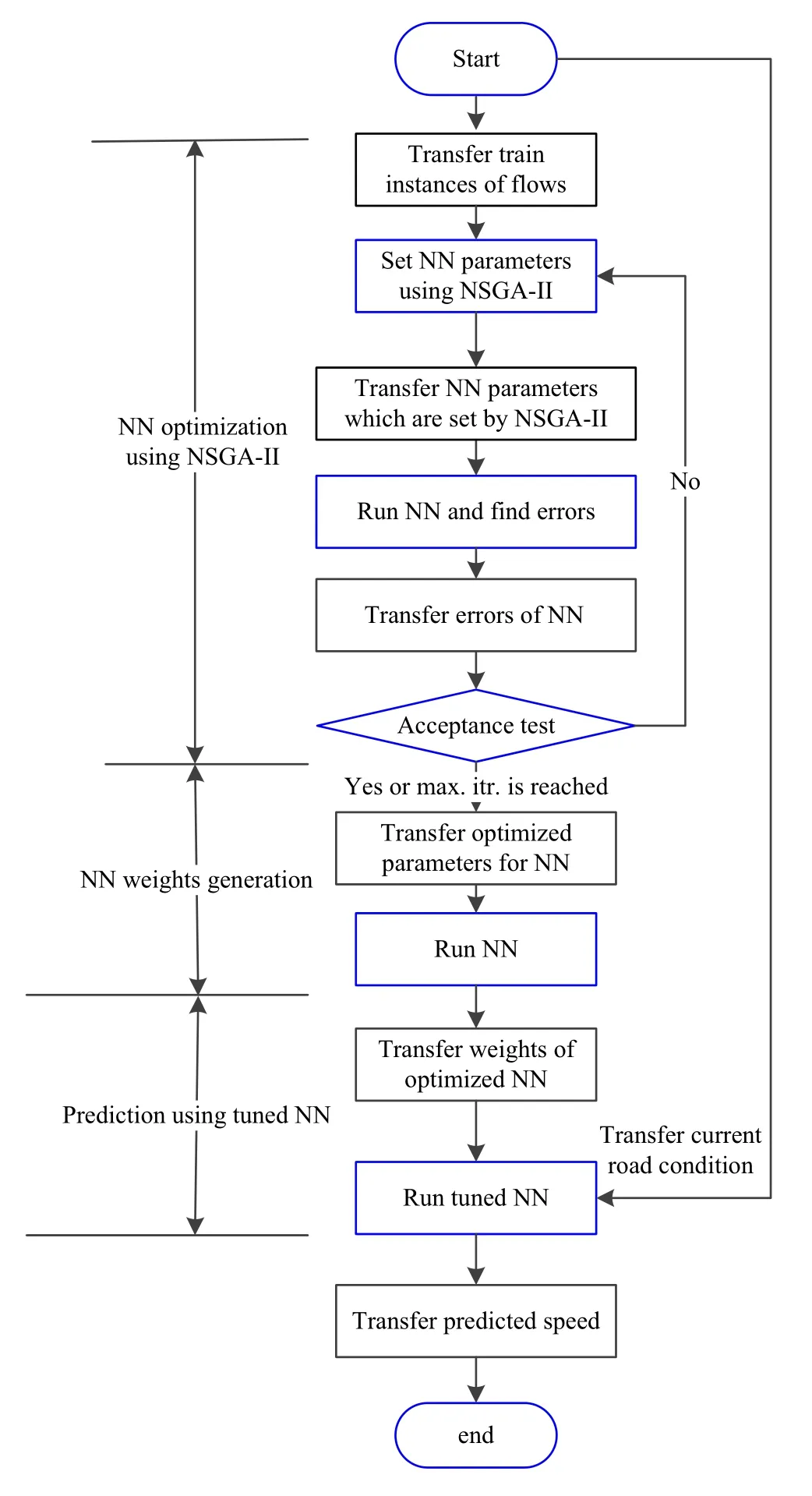
Fig. 2 Basic steps of optimizing multi-output MLP NN using NSGAII

4 Study data

As previously mentioned in Sect. 3, the proposed framework is self-adjusted and data-independent. So, it is expected to predict the traffic flow for each set of data regardless of the different situations. In order to test the framework with a comprehensive set of data, data were collected from a six-lane section along the Hashemi Rafsanjani Highway/Tehran with 1,500 m length for three consecutive typical days. Traffic behavior during 24 h on this highway includes both congested and non-congested hours. Graphical representation of the selected area and organization of the loop detectors are shown in Fig. 4.

The traffic flow data are collected from certain data collection points every 5 min. In this paper, data are normalized to values between 0 and 1. The data samples used for training, validation and testing of the NNs are normalized using the min-max normalization technique given as follows:

where Xnis the normalized value,and Xminand Xmaxare an instance of the minimum and maximum values of the vector to be normalized. This reduces the possibility of reaching the saturation regions of the sigmoid transfer function during training. Figure 5 shows the traffic flow data in the selected area, in 5-min resolution.

4.1 Temporal and spatial representation of data

In this section, different datasets used in this study are discussed. Finding a way of incorporating both temporal and spatial characteristics of traffic data time series is a worth mentioning issue. For example, consider the traffic flow series which varies as a function of time, V(t). Suppose that traffic data are collected using two detectors,one located in the desired section and the other one at the upstream. We name the data series collected by these detectors as Vdown(t) and Vup(t), respectively. In order to predict the value of Vdownat a given time t, the network must be trained using pairs of input-output values, where the input values could be

1. Time-lagged events of Vdown, such as Vdownt-1（ ），Vdownt-2（ ），...，Vdownt-n（ ）.

2. Time-lagged events of Vdownplus spatial attributes. In this case, input values are time-lagged events of both Vdownand Vup, such as Vdownt-1（ ），Vdownt-2（ ），...，Vdownt-n（ ），Vupt-1（ ），Vupt-2（ ），...，Vupt-n（ ）.

The first approach is considered as a univariate nonlinear prediction model, and the second one is a multivariate model.

The chosen highway section has three loop detectors:One is for collecting data at the desired section,and other two are placed at the upstream sections. Suppose that A and B represent the traffic data of the upstream sections(collected by No.02 and No.03 detectors, respectively)and C is for the downstream and the desired section(collected by No.01).

Using the following relationship between these time series,the model can easily carry out traffic data forecasts:

Obviously, when input values only contain temporal attributes, it does not contain A and B time series:

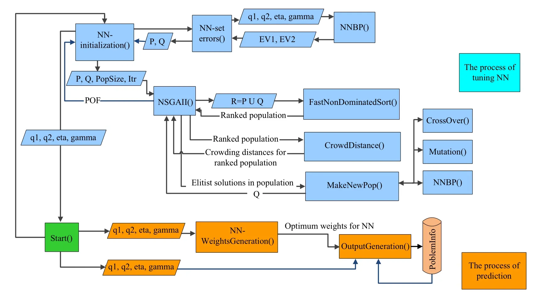
Fig. 3 The schematic representation of the optimization process

Fig. 4 Graphical representation of Hashemi Rafsanjani Highway

The main purpose of this paper is to discuss the optimization of NNs when we have more than one output.We also consider two input types containing temporal or spatiotemporal attributes. Here, network outputs will be one- and two-step-ahead predictions, which are the next 5 and 10 min. So simply assuming an MLP structure with two outputs, different types of input-output pairs used in this paper are as follows:

· Univariate (type 1 input):

· Multivariate (type 2 input):

4.2 Finding the input dimension

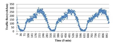
Fig. 5 Traffic flow behavior for 3 days

This section defines the aforementioned look-back window size or simply the input dimension. Increasing the input dimension of NNs can exponentially increase the computational complexity,but it may also increase the forecasting accuracy. Therefore, choosing the best dimension is a crucial issue. In this work, the statistical autocorrelation function (ACF) and partial autocorrelation function(PACF) are used for selecting the input dimension of a given time series in the nonparametric approach for traffic flow forecasting.Statistically,autocorrelation measures the degree of association between data in a time series separated by different time lags. The ACF is evaluated for various values of the lag time, and results are plotted. For traffic flows in 5-min intervals, the lag time will be in 5 min. Wherever the ACF curve intersects the lag time axis,its value is zero, indicating that y(t - D) and y(t) are linearly independent,where D denotes the look-back window size. The lag time corresponding to the first point of intersection is chosen as the optimum input dimension[19].

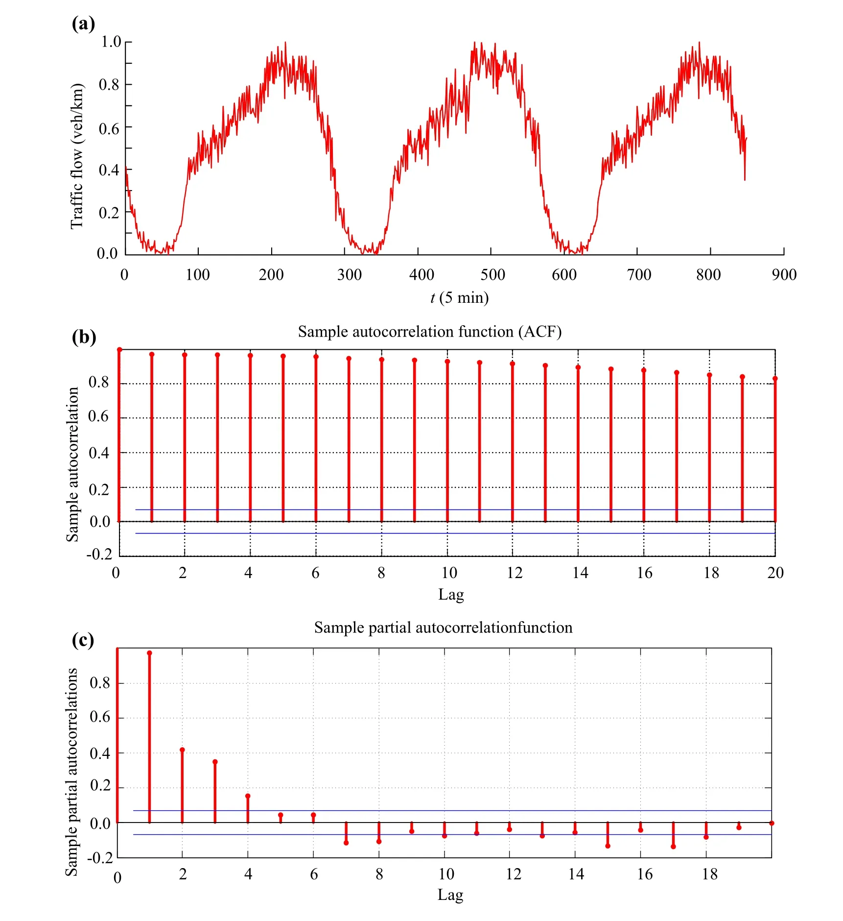
Fig. 6 Traffic flow measured in the selected two-lane freeway and its autocorrelation function:a time series plot,b autocorrelation histogram of the traffic flow data, and c partial autocorrelation histogram of the traffic flow data

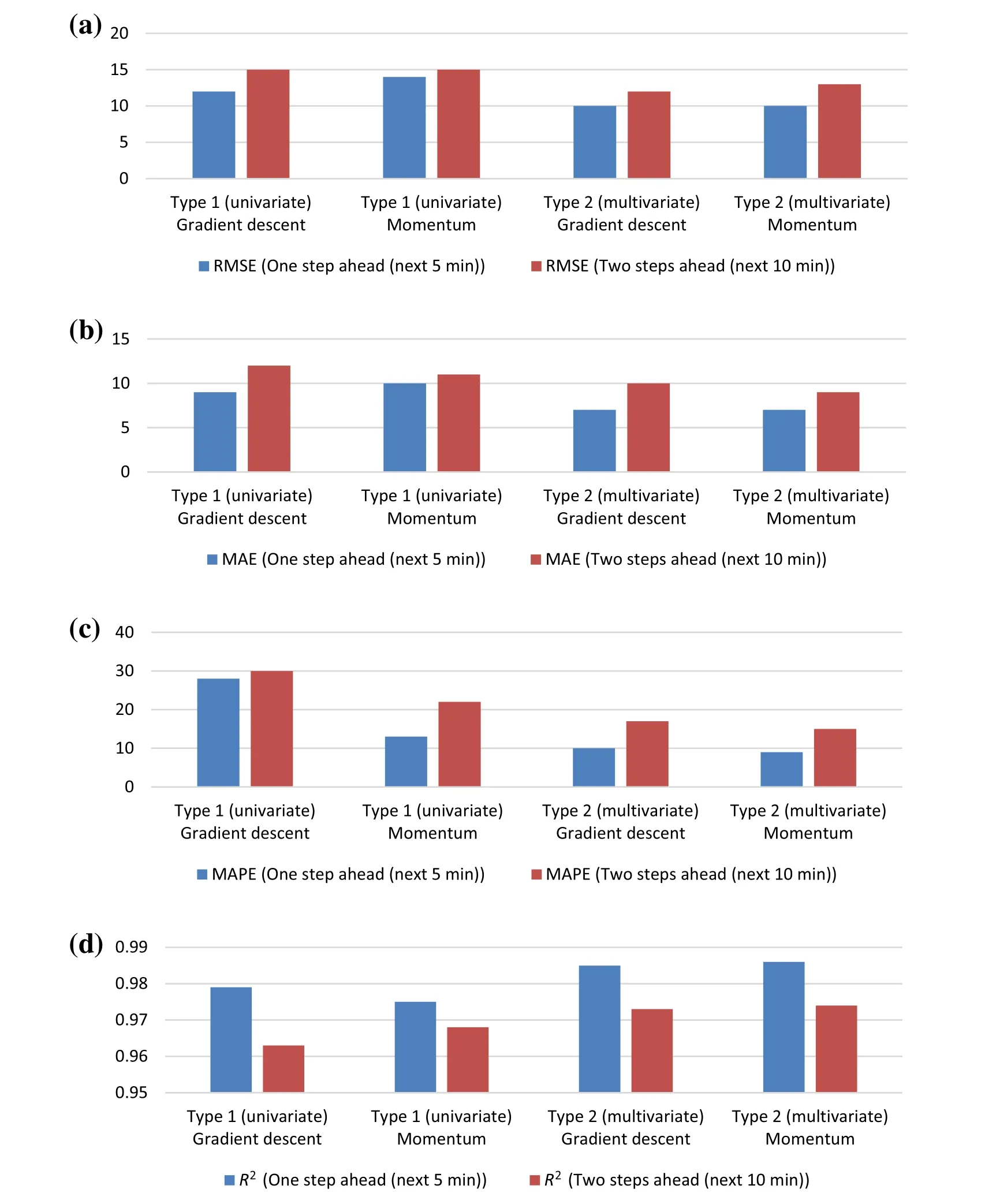
Fig. 7 Summary of the results: a RMSE values, b MAE values, c MAPE values, and d R2 values for different data types (univariate vs.multivariate), different learning algorithms (back-propagation with/without momentum) and different prediction horizons (5 min vs. 10 min ahead)

Table 1 Comparison results

Figure 6a shows the time series plot of 850 and 5-min traffic flow data continuously recorded over a period of 3 days, that is, the number of observations N = 850. It displays a strong seasonal periodical pattern of 24 h(1 day), as expected. Figure 6b shows the variation of the ACF for the shown traffic flow data in Fig. 6a, with a lag time of up to 20 (5-min). The autocorrelation plot shows that the sample autocorrelations are very strong and positive and decay very slowly.

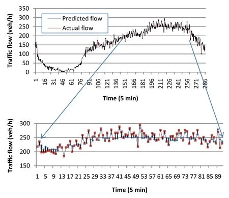
Fig. 8 Actual versus predicted flow of the univariate model for 5 min ahead

Fig. 9 Actual versus predicted flow of the univariate model for 10 min ahead

The next step is to produce the partial autocorrelation plot of the data.The partial autocorrelation plot of the data with 95% confidence bands shows that only the partial autocorrelations of the first,second,third and fourth lag are significant.

The PACF curve enters the confidence band at D = 4,indicating that y(t - 4) and y(t) are linearly independent.The lag time D = 4 is therefore chosen as the optimum value to be used in the input dimension (Fig. 6c).

In other words, a four-dimensional input traffic flow vector, including four time-lagged periods of flow from No. 01 and two output units (representing traffic flow for No. 01 at t + 1 and t + 2 time intervals), will be used to model the univariate set of data,and a six-dimensional input traffic flow vector, including four time-lagged periods of flow from No.01,one time-lagged periods of flow from both No.02 and No.03,and two output units(representing traffic flow for No. 01 at t + 1 and t + 2 time intervals), will be used to model the multivariate set of data.

5 Empirical results

In order to train and predict with NNs,50%of the available data is used for training, 25% for validation, and the rest 25% for testing. Mean square error (MSE) for validation data has been used as a measure of the network’s performance in the process of tuning NN. A set of elitist parameters are transferred to the next iteration; finally, the test data set is presented to the network to evaluate the performance of the adjusted network. Root mean square error (RMSE), mean average error (MAE) and the correlation coefficient known as R2, between the actual and predicted flow series,are the performance measures used to compare the predicted values against the actual values.These measures are defined in Eqs. (8)-(10):

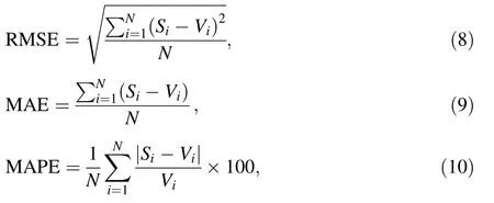
where Siis the predicted value for observation i, Viis the actual value for observation i, and N is the number of observations.

Prediction results are summarized in plots presented in Fig. 7.From the figures,all of the errors(MAE,RMSE and MAPE)are sufficiently small to show that NSGA-II can be used as a promising tool for optimizing NN’s parameters,with the aim of predicting the real-world traffic behavior.

Comparing errors in detail based on NN types, we find that using techniques like adding the momentum rate to the classic gradient descent method did not improve the performance.Both models have similar performance,and it is notable that the R2values in the models are very close and high for both one- and two-step-ahead predictions. Comparing errors based on data types (univariate and multivariate)shows that using spatial attributes in addition to the temporal ones improves the performance.

The aforementioned findings suggest that the multivariate approach can be used for traffic prediction at the selected highway site according to its predictive accuracy.

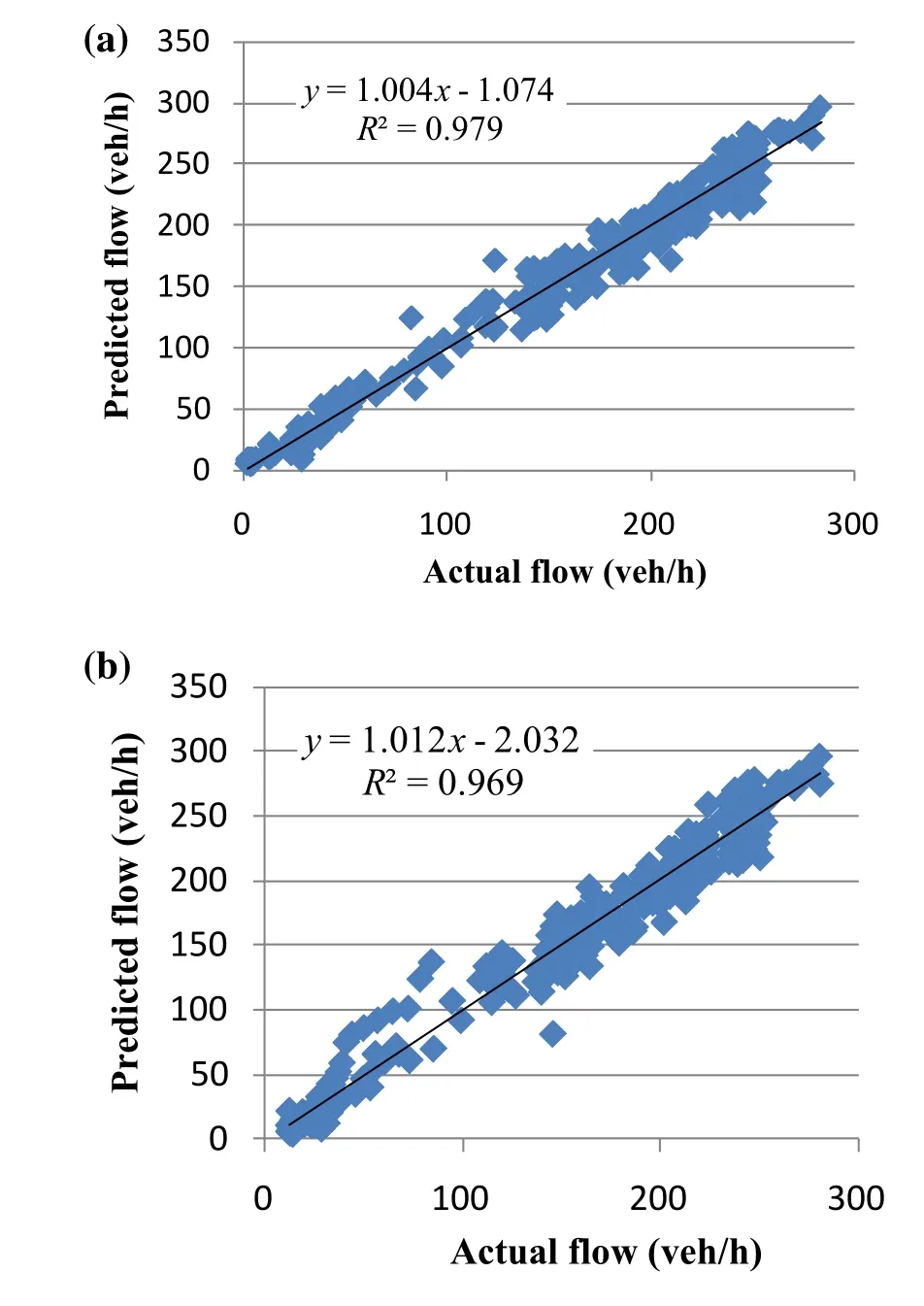
Fig. 10 Scatter plot of the univariate model:a 5 min ahead;b 10 min ahead

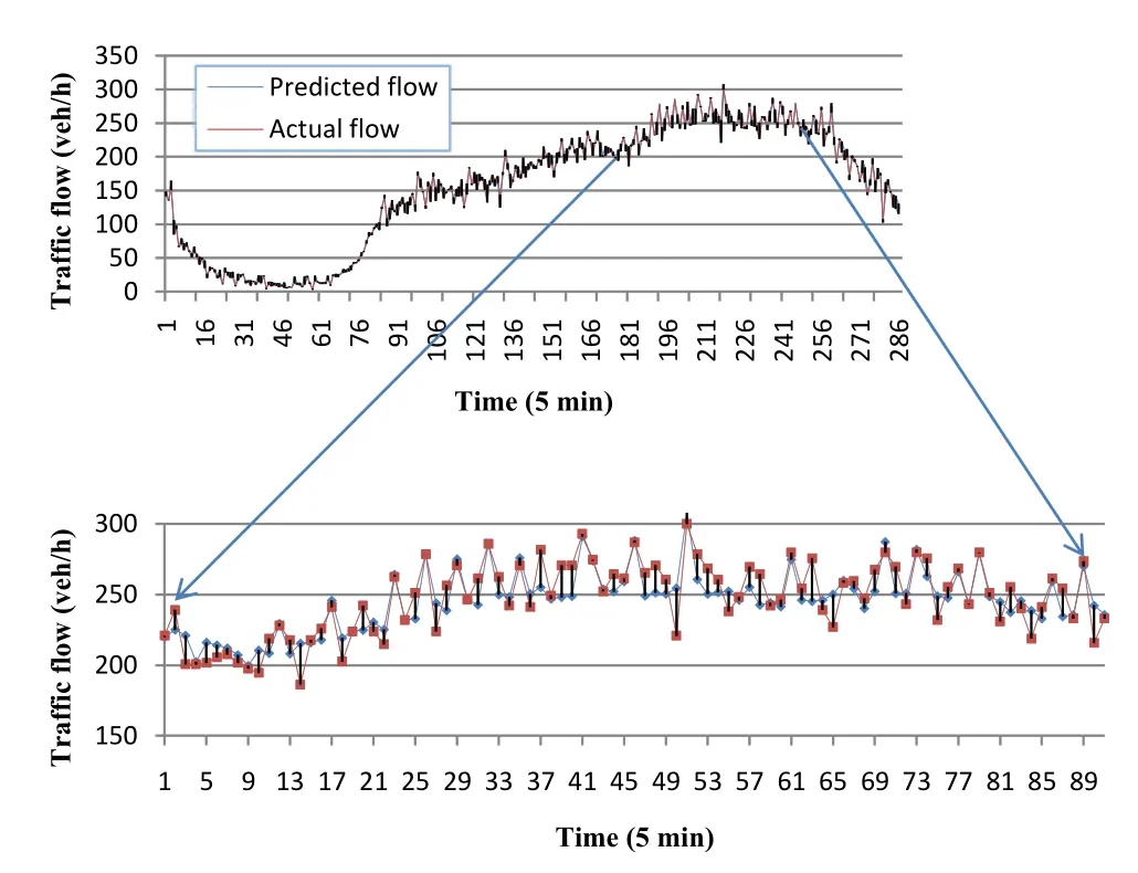
Fig. 11 Actual versus predicted flow of the multivariate model for 5 min ahead

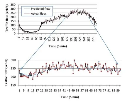
Fig. 12 Actual versus predicted flow of the multivariate model for 10 min ahead

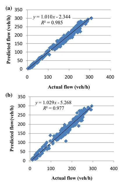
Fig. 13 Scatter plot of the multivariate model: a 5 min ahead;b 10 min ahead

In order to compare the accuracy of the proposed approach, multi-step-ahead prediction with the same data set is also provided with two other approaches:(1)seasonal ARIMA and (2) historical average. Table 1 shows the comparison results. MAPE and R2values are chosen to be reported for 10-min ahead prediction and with type 2 data as the models’ input. Our observations revealed that both the seasonal ARIMA and the optimized NN can achieve good forecast in application to traffic flow, but the developed predictive model using multi-output NN optimized with NSGA-II causes higher correlation between the predicted and actual traffic flows. This means that the traffic flow pattern predicted by the proposed approach is more coincident with the real traffic flow pattern.While the optimized NN results are comparable to the seasonal ARIMA, they both have better results than the simple historical average method.

Figures 8 and 9 show the predicted versus actual values of flow for the univariate model,for the next 5 and 10 min,respectively. Because of the similar results for both NNs,we only plot the results of genetically optimized gradient descent,for univariate and multivariate inputs.A portion of data points is magnified to clearly depict the differences.Figure 10 shows the scatter plot of the results shown in Figs. 8 and 9.

Similarly, Figs. 11 and 12 are for the multivariate approach and Fig. 13 shows the scatter plot.

6 Conclusion

The ability to predict the future values of traffic parameters helps to improve the performance of traffic control systems. Both single/multi-step-ahead predictions play a significant role in this field, but in cases of system failure,multi-step-ahead predicted values become beneficial. In order to avoid the low accuracy of long-term forecasts,instead of applying the iterated approach to the results of a single output model,multi-output NN is used in this study.This paper applied the NSGA-II to optimize the parameters of NNs with different learning rules and different types of inputs. This specific genetic algorithm is a well-known multi-objective genetic algorithm that finds a better spread of solutions in different problems.

The proposed framework predicts traffic flow values based on their recent temporal and spatial profiles at a given highway site during the past few minutes. Both temporal and spatial effects are found to be essential for more accurate prediction. Moreover, it was found that longer extent of prediction does not decrease the accuracy of results in this model. The model performance was validated using real traffic flow data obtained from the field.

This paper demonstrates the ability of this class of genetic algorithms to produce the best combination of network parameters.Results obtained from test data adduce that the model generalization ability is satisfactory.For the case of 5-and 10-min prediction horizon, R2indices are at least 0.98,which evidently shows the model generalization ability.

Open AccessThis article is distributed under the terms of the Creative Commons Attribution 4.0 International License (http://creativecommons.org/licenses/by/4.0/), which permits unrestricted use,distribution,and reproduction in any medium,provided you give appropriate credit to the original author(s) and the source, provide a link to the Creative Commons license, and indicate if changes were made.