Numerical Modeling Strategy for the Simulation of Nonlinear Response of Slender Reinforced Concrete Structural Walls

MohammedA.MohammedandAndreR.Barbosa,

Abstract: A three-dimensional nonlinear modeling strategy for simulating the seismic response of slender reinforced concrete structural walls with different cross-sectional shapes is presented in this paper.A combination of nonlinear multi-layer shell elements and displacement-based beam-column elements are used to model the unconfined and confined parts of the walls,respectively.A uniaxial material model for reinforcing steel bars that includes buckling and low-cyclic fatigue effects is used to model the longitudinal steel bars within the structural walls.The material model parameters related to the buckling length are defined based on an analytical expression for reinforcing steel bars embedded in reinforced concrete elements,which are developed based on beam-on-springs model,and validated with experimental tests of boundary elements of structural walls available in the literature.Six experimental case studies of reinforced concrete walls with rectangularshape,T-shape,and U-shape cross-section are used to validate the structural wall numerical modeling strategy.

Keywords: Bar buckling,finite element modeling,low-cycle fatigue,reinforced concrete structural walls.* Corresponding Author:Andre R.Barbosa.Email:andre.barbosa@oregonstate.edu.

1 Introduction

Slender reinforced concrete (RC) walls are one of several possible structural elements used to resist lateral loads in mid-rise and high-rise RC buildings.The cross-section of these elements can be rectangular or non-rectangular,e.g.,with T-shape or U-shape.The nonlinear response simulation of non-rectangular cross-section walls is more complex than the nonlinear simulation of walls with rectangular cross-section,mainly because of nonuniform axial strain distribution in compression and tension of the wall cross-section due to shear lag [Beyer,Dazio and Priestley (2008);Lu and Panagiotou (2016)].In addition,the interaction between axial,flexural,and shear loading generates multi-axial stress and strain states that need to be accounted for in the nonlinear modeling of the concrete and reinforcing steel bar materials.

Laboratory testing [Thomsen and Wallace (2004);Beyer,Dazio and Priestley (2008);Dazio,Beyer and Bachmann (2009)] and post-earthquake observations [Lowes,Lehman,Birely et al.(2012)] have shown that well-detailed slender RC walls tend to concentrate damage at the wall ends (boundary elements) of the wall plastic hinge,when special detailing procedures are followed.The three main modes of damage typically observed in the wall boundary elements include reinforcing steel bar buckling,bar rupture due to lowcyclic fatigue,and concrete crushing.Considering the non-rectangular cross-section walls,the finite element (FE) models should be able to predict the cyclic response of RC walls under combined effects of axial,shear,and bending,the buckling and low-cycle fatigue failures of the reinforcing steel bars were not simulated in these models.

With respect to inelastic modeling of RC structural walls,the models that exist in the literature that can be classified as:(1) macro models and (2) micro models.Lumped plasticity models are considered to be the simplest and most basic macro modeling approach to capture the nonlinear response [Panneton,Leger and Tremblay (2006);Ghorbanirenani,Velev,Tremblay et al.(2009);Boivin and Paultre (2010);Rejec,Isakovic and Fischinger (2012)].Lumped plasticity models consist of a flexural hinge at the base of the wall in which the critical section of the wall is located,while the remaining part of the wall is simulated using linear elastic elements.A predefined moment-rotation backbone curve is assigned to the flexural hinge that controls the nonlinear behavior of the wall.Although this type of modeling is numerically robust and computationally efficient,this model is only useful for very limited cases of cyclic response prediction due to the predefined moment-rotation relationship that are greatly dependent on empirical calibration.

Distributed plasticity models such as fiber section beam-column elements (line elements) have been used extensively to study the nonlinear behavior of the slender structural walls [Ranzo and Petrangeli (1998);Barbosa,Panagiotou,Conte et al.(2009);Martinelli and Filippou (2009);Boivin and Paultre (2012);Pugh,Lowes and Lehman (2015)].The distributed plasticity elements provide multiple regions along the height of the structural walls where the nonlinear response can be captured.While the line elements provide simple and robust way to model the nonlinear response of structural walls,the limitation when simulating nonlinear response of non-rectangular structural walls (e.g.,T-shape and Ushape walls) are well known.In addition,regularization procedures similar to the one in [Barbosa (2009);Barbosa,Panagiotou,Conte et al.(2009);Pugh,Lowes and Lehman (2015)] are needed to improve the accuracy of response predictions.

Orakcal et al.[Orakcal,Wallace and Conte (2004);Orakcal,Massone,Wallace et al.(2006)] and Kolozvari et al.[Kolozvari,Orakcal and Wallace (2015);Kolozvari,Arteta,Fischinger et al.(2018)] used an enhanced version of the multiple-vertical-line-element model (MVLEM) that was developed in Vulcano et al.[Vulcano,Bertero and Colotti (1988)] to simulate the nonlinear response of slender structural walls with rectangular cross-section.The MVLEM model consists of multiple line elements with horizontal springs at specific height,which are used to capture the shear behavior of the wall.This model has been used in several previous studies to model the flexural and shear response of structural walls.

Barbosa [Barbosa (2011)] and Lu et al.[Lu and Panagiotou (2016)] used three dimensional nonlinear beam-truss modeling (BTM) approach to simulate the inelastic response of structural walls.The BTM approach includes explicitly the flexure-shear interaction and is able to also capture the diagonal shear failure of the structural walls.Additionally,this approach can be used to simulate the nonlinear behavior of structural walls with different geometrical sections (U-shape,I-shape and T-shape walls) [Lu and Panagiotou (2016)].However,this approach also requires detailed regularization procedures and is more computationally expensive and has higher level of complexity compared with other macro models described previously.

In the realm of micro modeling approaches,two-dimensional (2-D) and three-dimensional (3-D) continuum FE models with shell,plate,and solid elements have been shown to be able to capture the nonlinear behavior and failure modes of structural walls.Using such approaches for modeling can improve the accuracy of the predicted response and overcome limitations of using macro modeling approaches.However,this type of modeling is more complicated and the type of the elements that are used for the analyses in this approach are computationally demanding.Palermo and Vecchio [Palermo and Vecchio (2002)] used 2-D plane stress elements with a 2-D reinforced concrete constitutive model based on the modified compression field theory (MCFT) to achieve accurate simulation of RC walls tested by them.Lehman et al.[Lehman,Lowes,Pugh et al.(2015)] used three-dimensional brick elements with a continuum damage concrete model with fixed orthogonal crack model to study the monotonic response of different structural RC walls available in the literature.Dashti et al.[Dashti,Dhakal and Pampanin (2017)] used curved shell elements with embedded reinforcing bars to develop FE models of rectangular RC structural walls.

Lu et al.[Lu,Guan,Huang et al.(2015)] developed a quadrilateral multi-layer shell element model that incorporates 2-D concrete material constitutive models.The shell element was implemented as a shell element with multi-layered section.The shell element accounts for large deformation by using the updated Lagrangian formulation.Lu et al.[Lu,Guan,Huang et al.(2015)] validated the shell element and material model against several RC wall tests and used it to study the nonlinear response of super-tall buildings with structural walls.Although the developed FE models described in this paragraph were able to predict the cyclic response of RC walls under combined effects of axial,shear,and bending,the buckling and low-cycle fatigue failures of the reinforcing steel bars were not simulated in these models,and care should be taken with respect to regularization of the concrete material crushing response.

Most of the reinforcing steel bar material models available in the literature that capture the effect of bar buckling are based on the assumption that the buckling length of reinforcing steel bars is limited to one tie spacing and do not consider the effect of bar embedment [Brelser and Gilbert (1961);Monti and Nuti (1992);Gomes and Appleton (1997);Kunnath,Heo and Mohle (2009);Mendes and Castro (2014);Kashani,Lowes,Crewe et al.(2015);Kim and Koutromanos (2016)].However,experimental studies and observed damage in real structural elements following earthquakes have shown that the buckling length can extend over more than one tie spacing and that the effect of longitudinal bar embedment and of the stiffness of transverse reinforcement can play an important role in the performance and failure of reinforced concrete walls [Thomsen and Wallace (2004);Dazio,Beyer and Bachmann (2009)].Therefore,models that capture buckling behavior of reinforcing steel bars should include these effects.

The modeling of embedded bars has also been studied in detail over the last couple of decades [Dhakal and Maekawa (2002);Eom,Kang,Park et al.(2014);Su,Wang,Bai et al.(2015)].Dhakal and Maekawa [Dhakal and Maekawa (2002)] developed an analytical method to predict the buckling length of reinforcing steel bars inside reinforced concrete members.This method used the principal of minimum potential energy to determine the minimum required lateral stiffnessKeqto prevent buckling of the reinforcing steel bar.The minimum required lateral stiffness is determined as the ratio of the stiffness of the lateral tiesKtover the stiffness of the longitudinal reinforcing steel barKwhich is a function of the flexural rigidity (EI) of the longitudinal reinforcing steel bar,asK=EIπ4/S3,where,fyis the yield stress in MPa,Sis the tie spacing in mm,Esis the Young’s modulus of the reinforcing steel bars,andIis the nominal second moment of inertia of the bars.Eom et al.[Eom,Kang,Park et al.(2014)] performed a parametric study to estimate the reduced modulus of longitudinal reinforcing steel bars undergoing post-yield buckling.In this study,the value ofEris determined byEr= 2.87Et,whereEtandErare the hardening tangent modulus and reduced modulus of longitudinal reinforcing steel bar,respectively.The critical post-yield buckling stress of the longitudinal reinforcing steel bar is based on the value of the reduced modulus.Su et al.[Su,Wang,Bai et al.(2015)] used a beam-on-springs model to estimate the buckling length of longitudinal reinforcing steel bars following the approach in Dhakal et al.[Dhakal and Maekawa (2002)].However,a different value for the effective modulus of elasticity of the reinforcing steel was used that is given byE=αtEt+ (1 -αt)Er.The coefficientαtaccounts for the engaged portion of the tangent modulus and is calibrated using a large experimental dataset.

Only a few models available in the literature provide the compression stress-strain envelope for buckled reinforcing steel bars [Zong,Kunnath and Monti (2014);Massone and Lopez (2014)].Zong et al.[Zong,Kunnath and Monti (2014)] developed a stress-strain relationship for reinforcing steel bars in compression based on a simplified bar with springs model,which accounts for the effects of buckling and transverse reinforcements under monotonic loading.The model was validated only using results from FE analyses.Massone et al.[Massone and Lopez (2014)] developed a four plastic hinge reinforcing steel bar model that was adjusted according to the distribution of the transverse reinforcement to study the global buckling effects of reinforcing steel bars.This model cannot be used as a uniaxial material in the framework of FE analysis due to fact that the developing of this model was at the element level and not at the material level.All the models that are mentioned above were developed mainly to predict the critical load and the buckling length.

For nonlinear FE models of structural walls,previous studies [Rots,Nauta,Kuster et al.(1985);Barbosa,Panagiotou,Conte et al.(2009);Pugh (2012);Lehman,Lowes,Pugh et al.(2015)] showed that the simulated softening response and strength loss of compression controlled concrete components are affected by the element size and softening of the material model.Therefore,a regularization procedure is required to obtain objective responses.In general,objective responses can be achieved by calibrating the concrete material models in terms of fracture and crushing energy and characteristic element sizes.The main objective of this study is to develop a FE modeling strategy that allows for the simulation of the nonlinear response of slender RC walls with different geometric shapes and captures failure modes associated with reinforcing steel bar buckling and low-cycle fatigue.The modeling strategy consists of a combination of displacement-based beamcolumn (DBBC) fiber-section elements and multi-layer shell (MLS) elements.Uniaxial and two-dimensional constitutive material models are used to model the nonlinear response of the concrete of the fiber-sections of the DBBC and MLS elements,respectively.The DBBC elements are used to model boundary elements and corners of the walls and the MLS elements are used to model the rectangular parts of the walls.

The paper is divided into four sections.In Section 2,an analytical model developed to predict the buckling length of reinforcing steel bars embedded in RC elements is presented,and validated for use in fiber-sections of wall boundary elements.Section 3 describes the strategy developed for modeling the cyclic response of structural walls,including a regularization procedure to adjust for mesh size effects of the MLS elements.In Section 4,six case studies of slender RC walls with R-shape,T-shape,and U-shape sections are analyzed to test and validate the efficacy and accuracy of the numerical modeling strategy developed.Finally,Section 5 provides the conclusions and limitations of this study.In addition,suggestions for future work are provided in this last section.

2 Buckling length model for reinforcing steel bar embedded in reinforced concrete elements

A beam-on-springs model subjected to compression axial loads is used to develop an analytical model to estimate the buckling length.Fig.1(a) shows the beam-on-springs model that is used in this study.The open source FE analysis platform,OpenSees [PEER (2016);Open System for Earthquake Engineering Simulation] is used to develop the beamon-springs model.This model consists of an isolated reinforcing steel bar modeled with DBBC elements and supported laterally by a series of zero-length spring elements.The OpenSeesSteel4uniaxial material [Zsarnoczay (2013)] is used to model the uniaxial response of the isolated bar.Additionally,the corotational formulation is used to capture the geometric nonlinearity.The reinforcing steel bar at both ends is restrained against any rotation degree of freedom and any translation perpendicular to the bar axis.A displacement control integrator and the Krylov-Newton algorithm [Scott and Fenves (2009)] are used to solve the nonlinear system of static equilibrium equations in the pushdown analysis.The norm of displacement increment test with a tolerance equal to 10-8and a maximum number of iterations equal to 20 are used for convergence checks during the numerical solution.Based on results of a preliminary set of analyses performed on the isolated bar model it was found that:(1) the response of the model in terms of initiation of the buckling,maximum strength capacity,and residual strength converged with circular section mesh with 36 fibers in the circumference direction and 6 fibers in the radial direction;(2) elements with a length equal to 10 mm,and with two integration points,produced a converged buckling response;and (3) to initiate buckling,an initial lateral displacement imperfection of 1.0 ×10-6of the bar length is applied at the mid-height of the model.Based on work of Eom et al.[Eom,Kang,Park et al.(2014)],a linear effective stiffness,Kspring,is assigned as a tension material constant for each spring in the transverse direction of the bar to model the effects of the transverse reinforcement.The distance between two successive springs represents the tie spacing (S) in a RC element.An extremely large value (2.0 ×108N/mm) of the stiffness is assigned for the compressive side of the transverse springs to prevent the inward buckling and to control the expected direction of buckling.

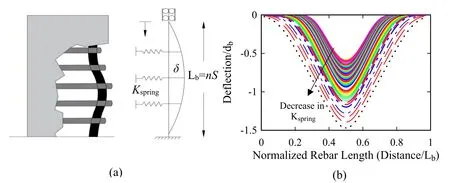
Figure 1:Beam on springs model:(a) FE model (b) parametric study sample results of the effect of on the buckling (lateral) modes

A parametric study with over 300 analyses is performed using the beam-on-springs model with varying values of lateral stiffness for the springs.The objective of this parametric study is to investigate the relationship between the lateral stiffness of the springs and the developed buckling length of the reinforcing steel bars.Fig.1(b) shows a sample of the obtained buckling length of reinforcing steel bars with different values ofKspringas obtained from the parametric analysis.Several observations can be made based on the results from the analyses of the beam-on-springs model.First,it was found that the required stiffness (Kspring) and flexural rigidity valuesdeveloped in Dhakal et al.[Dhakal and Maekawa (2002)] are accurate to obtain a buckling length equal toS.However,the Dhakal et al.[Dhakal and Maekawa (2002)] model overestimated the value ofKspringwhen predicting buckling lengths greater thanS.Instead,by using the values for flexural rigidity (EI= 2.87EtI) proposed in Eom et al.[Eom,Kang,Park et al.(2014)] to estimate the lateral stiffness,the beam-on-springs model was able to predict buckling lengths greater thanS.

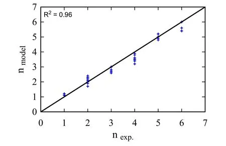
Figure 2:Relation and coefficient of determination between ne xp and nm odel

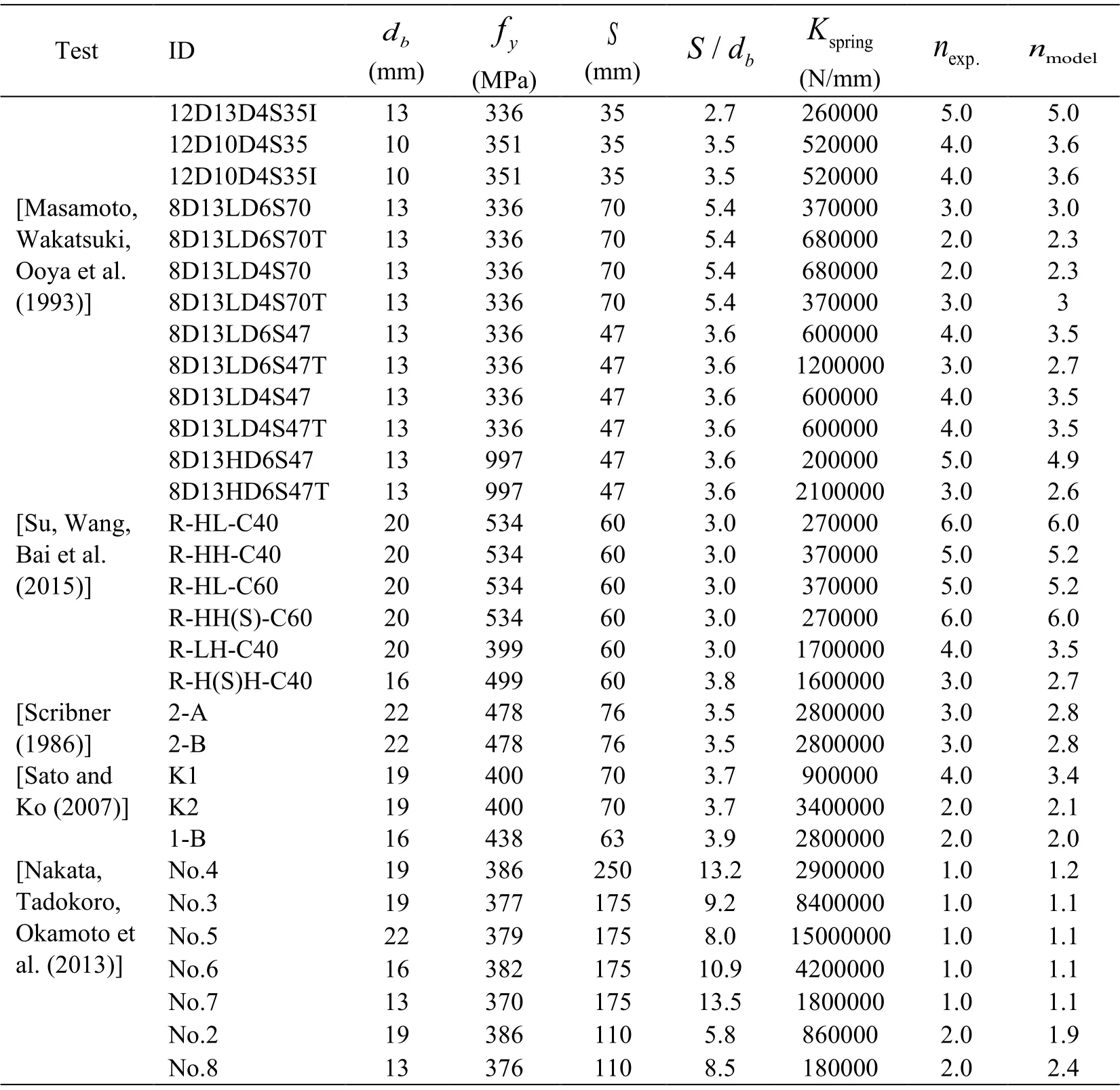
To validate the findings from the parametric study,the reported buckling length from an experimental dataset of 77 rectangular columns [Scribner (1986);Masamoto,Wakatsuki,Ooya et al.(1993);Kato and Ooya (1993);Ooya and Kato (1994);Kato,Kanaya and Wakatsuki (1995);Sato and Ko (2007);Nakata,Tadokoro,Okamoto et al.(2013);Su,Wang,Bai et al.(2015)] is used to compute the value ofKspringassigned to the FE model.This dataset was also used in Dhakal et al.[Dhakal and Maekawa (2002)] and Su et al.[Su,Wang,Bai et al.(2015)] to develop an analytical model to predict the buckling length of embedded reinforcing steel bars.Then,the results from the FE beam-on-springs model is compared with the observed buckling length from the experimental dataset.Tab.1 summarizes the results of the computation of the buckling length measured as the number of tie spacings for the model,nmodel,and the corresponding one observed in the experiment,nexp.Note that thenexpvalues are reported as buckling modes observed from the experiment (nmodel=1,2,etc.).On the other hand,nmodelis calculated by plotting the deflected shape of the reinforcing steel bar model and measuring the corresponding buckling length.Fig.2 shows the correlation between the computed values for the buckling length obtained from the analyses and the one obtained from the experimental tests,where i t can be seen that the beam-on-springs model can predict accurately the observed buckling length (R2= 0.96) that is measured from the experimental dataset.

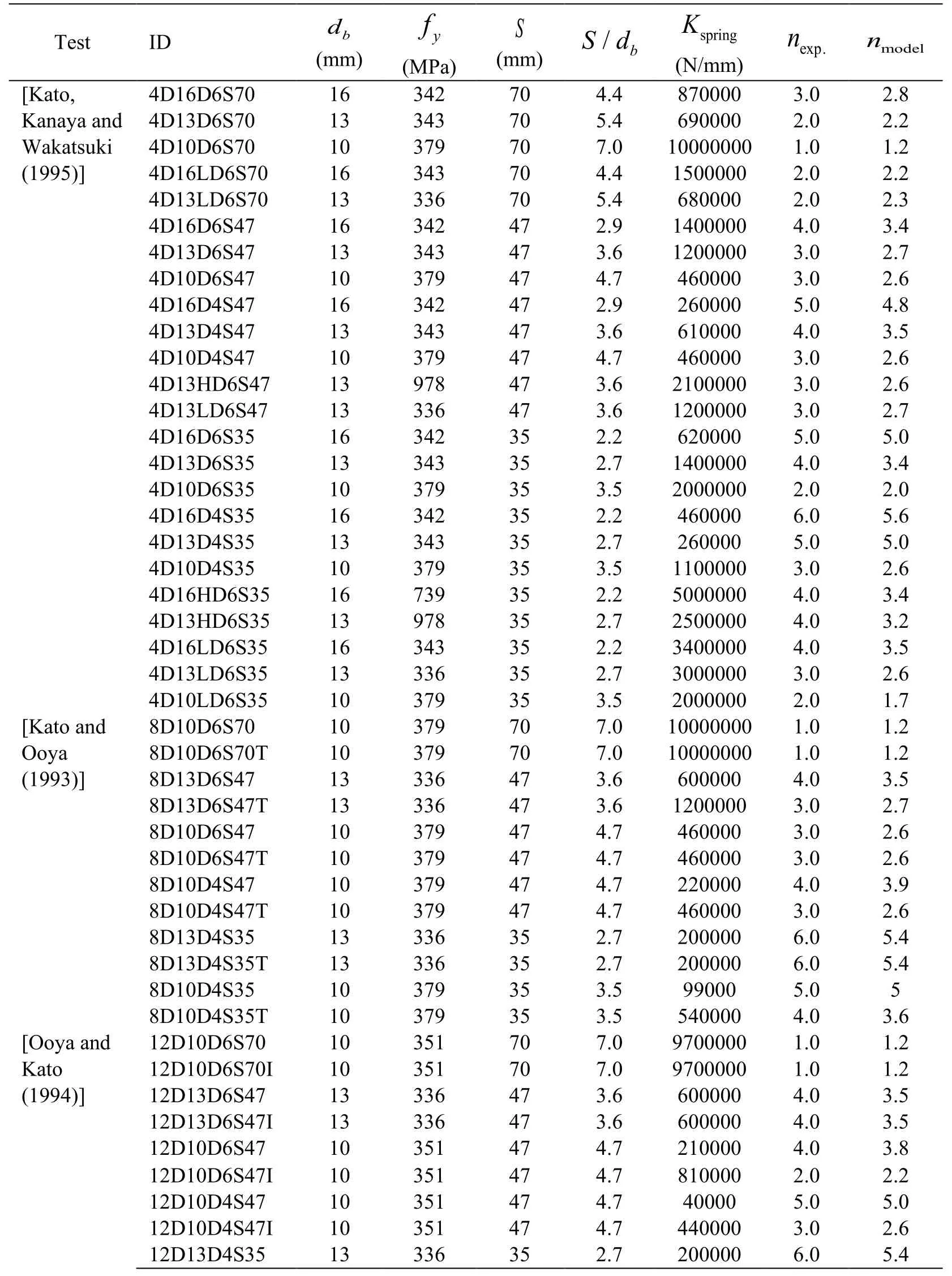
Table 1: Buckling length to spacing ratio from the beam-on-springs model and experiments

Test ID (m dm b ) (M fPy a ) (mS m ) S / d b (KN/ smprimng) ne xp. nm odel 12D13D4S35I 13 336 35 2.7 260000 5.0 5.0 12D10D4S35 10 351 35 3.5 520000 4.0 3.6 12D10D4S35I 10 351 35 3.5 520000 4.0 3.6 [Masamoto,8D13LD6S70 13 336 70 5.4 370000 3.0 3.0 Wakatsuki,8D13LD6S70T 13 336 70 5.4 680000 2.0 2.3 Ooya et al.8D13LD4S70 13 336 70 5.4 680000 2.0 2.3 (1993)] 8D13LD4S70T 13 336 70 5.4 370000 3.0 3 8D13LD6S47 13 336 47 3.6 600000 4.0 3.5 8D13LD6S47T 13 336 47 3.6 1200000 3.0 2.7 8D13LD4S47 13 336 47 3.6 600000 4.0 3.5 8D13LD4S47T 13 336 47 3.6 600000 4.0 3.5 8D13HD6S47 13 997 47 3.6 200000 5.0 4.9 8D13HD6S47T 13 997 47 3.6 2100000 3.0 2.6 [Su,Wang,R-HL-C40 20 534 60 3.0 270000 6.0 6.0 Bai et al.R-HH-C40 20 534 60 3.0 370000 5.0 5.2 (2015)] R-HL-C60 20 534 60 3.0 370000 5.0 5.2 R-HH(S)-C60 20 534 60 3.0 270000 6.0 6.0 R-LH-C40 20 399 60 3.0 1700000 4.0 3.5 R-H(S)H-C40 16 499 60 3.8 1600000 3.0 2.7 [Scribner 2-A 22 478 76 3.5 2800000 3.0 2.8 (1986)] 2-B 22 478 76 3.5 2800000 3.0 2.8 [Sato and K1 19 400 70 3.7 900000 4.0 3.4 Ko (2007)] K2 19 400 70 3.7 3400000 2.0 2.1 1-B 16 438 63 3.9 2800000 2.0 2.0 [Nakata,No.4 19 386 250 13.2 2900000 1.0 1.2 Tadokoro,No.3 19 377 175 9.2 8400000 1.0 1.1 Okamoto et No.5 22 379 175 8.0 15000000 1.0 1.1 al.(2013)] No.6 16 382 175 10.9 4200000 1.0 1.1 No.7 13 370 175 13.5 1800000 1.0 1.1 No.2 19 386 110 5.8 860000 2.0 1.9 No.8 13 376 110 8.5 180000 2.0 2.4

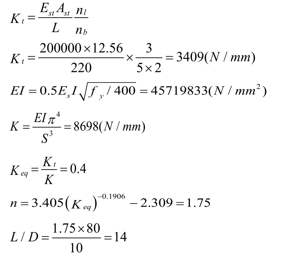
Based on the results from the parametric study,a regression analysis using a power law (see Fig.3) was used to develop an analytical model for predicting the buckling length of reinforcing steel bars embedded in RC structural elements.The buckling length (Lb=ns) described as a function of the number of transverse bar spacing is given by:

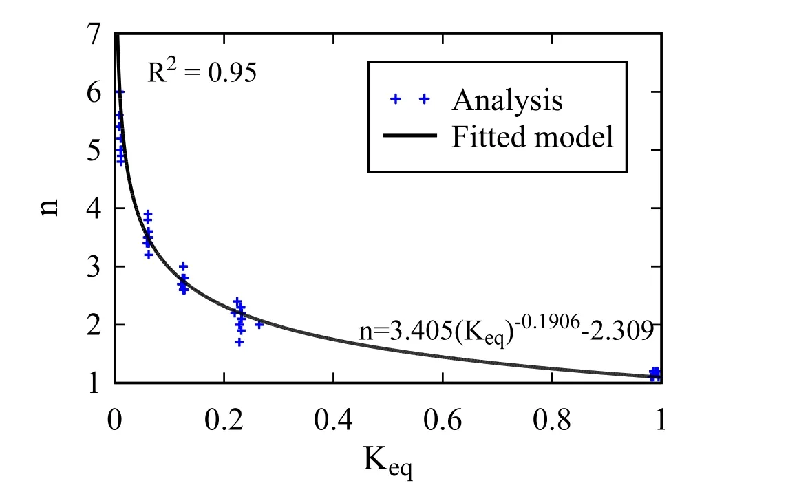
Figure 3:Beam on springs model and fitted analytical model results for buckling length normalized by the tie spacing versus the equivalent tie stiffness

whereKtrepresents the axial stiffness of the ties that support the longitudinal reinforcing steel bar;Kis the longitudinal reinforcement buckling stiffness;Est,Ast,andLare the elastic modulus,cross sectional area,and length of the ties;nlandnbare the number of ties and the number of supported longitudinal bars,respectively;EsandIare the elastic modulus and the moment of inertia of the longitudinal bars,respectively;the value offyin Eq.(5) is in MPa.Note that the range of validitynin Eq.(1) is limited to seven,because the proposed beam-on-springs model was only validated with experimental dataset where the observed buckling length was limited to seven tie spacings.

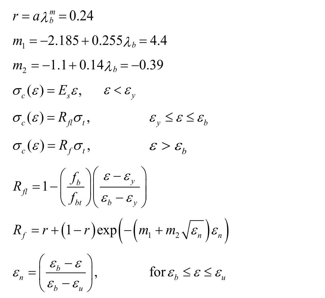
The modeling for buckling length of reinforcing steel bars embedded in RC elements developed above is validated using experimental test results of RC members presented in Taleb et al.[Taleb,Tani and Kono (2016)] and Welt et al.[Welt,Massone,Lafave et al.(2017)].In total,five specimens representing boundary elements of RC walls with different levels of confinement tested under monotonic compression load are used to validate the use of the analytical buckling length model in assigning parameters to the reinforcing steel uniaxial material model used in fiber-section modeling of RC members under compression.The FE models are developed in OpenSees to simulate the nonlinear response of the tested boundary elements.A force-based element with five Gauss-Lobatto integration points is used to model the RC boundary element.Unconfined and confined concrete material models parameters are assigned for the cover and core concrete fibers,respectively.The Scott-Kent-Park uniaxial material model available in OpenSees asConcrete02is used to model the nonlinear behavior of the concrete fibers.The concrete confinement parameters are calculated using Mander et al.[Mander,Priestley and Park (1988)].A uniaxial material model developed by the authors (see Appendix A),which accounts for buckling and lowcycle fatigue effects,is used to model the reinforcing steel bars.TheSteel4material model is used as the base for the developed reinforcing steel material model.The compression response of the developed uniaxial material model can be defined in terms of a nondimensional parameter λbgiven by:

Tab.2 summarizes the parameters used for the validation analyses and Tab.3 summarizes the parameters used to generate the compression envelope of the reinforcing steel bars for all specimens.Appendix B provides an example application for the ID4 test,listed in Tab.2,on the determination of the embedded reinforcing steel bar buckling length.

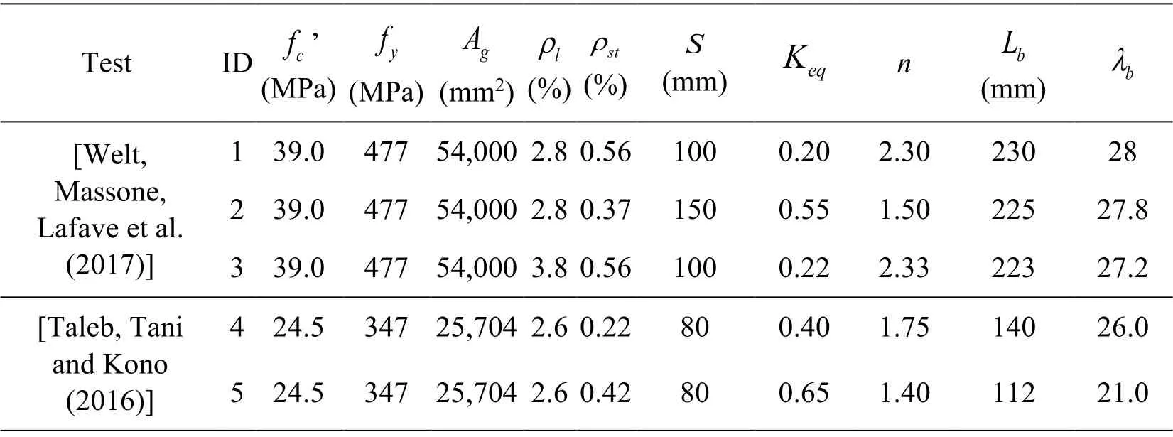
Table 2:Parameters used for validation analyses of the reinforcing steel bar model embedded in boundary elements tested under compression loading

Table 3:Steel4 model parameters used for validation analyses of the reinforcing steel bar model embedded in boundary elements tested under compression loading

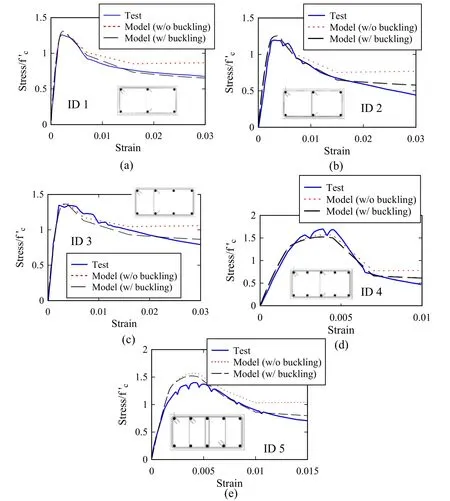
Figure 4:Effect of modeling reinforcing steel bar buckling for tests listed in Tab.2 using the buckling length model developed:(a) Test ID 1 (b) Test ID 2 (c) Test ID 3 (d) Test ID 4 (e) Test ID 5

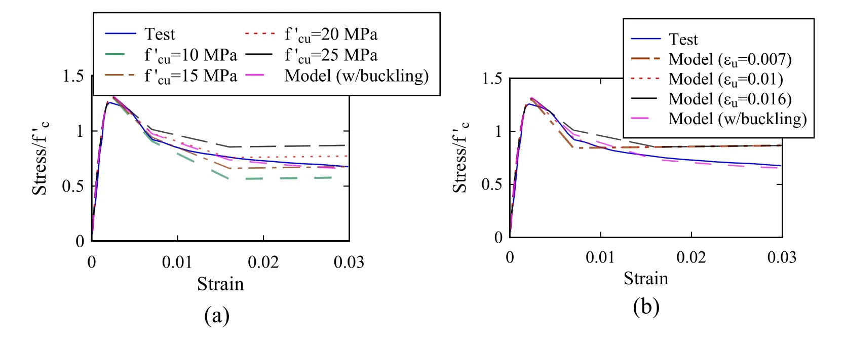
Figure 5:Specimen ID 1 model response sensitivity to different values of concrete uniaxial material model parameters (a) ultimate stress, (b) ultimate strain,

Fig.4 shows the effect of modeling the reinforcing steel bar buckling for tests listed in Tab.2 using the buckling length model in Eq.(1).Results indicate that the models without the effect of reinforcing steel bar buckling overestimate the predicted residual strength for all specimens.On the other hand,when the effect of reinforcing steel bar buckling is included in the analysis,the models are able to predict the softening response of the specimens with smaller error.The obtained mean absolute percentage errors of the softening part for the five specimens range from 3.3% to 10.0%,for the responses shown.Naturally,there are other RC modeling parameters that also contribute to the softening response and estimate of the residual strength.Fig.5(a) and Fig.5(b) show the effects of using different ultimate stress and strain values for the concrete model,respectively,on the predicted residual strength of specimen (ID 1) without including the reinforcing steel bar buckling effect in the models.Results in these figures indicate that the inclusion of the bar buckling model provides best results.

3 Nonlinear numerical strategy for slender RC walls

3.1 Element discretization

Fig.6 shows the framework for the numerical approach used in this study to model slender RC walls accounting for potential reinforcing steel bar buckling at boundary elements.The modeling strategy consists of using displacement-based beam-column (DBBC) elements and multi-layer shell (MLS) elements.First,the DBBC elements with nonlinear fibersection are used to model the boundary elements as well as the wall corners.At each integration point,the cross-section of the element is divided into fibers to which nonlinear uniaxial material models are assigned.

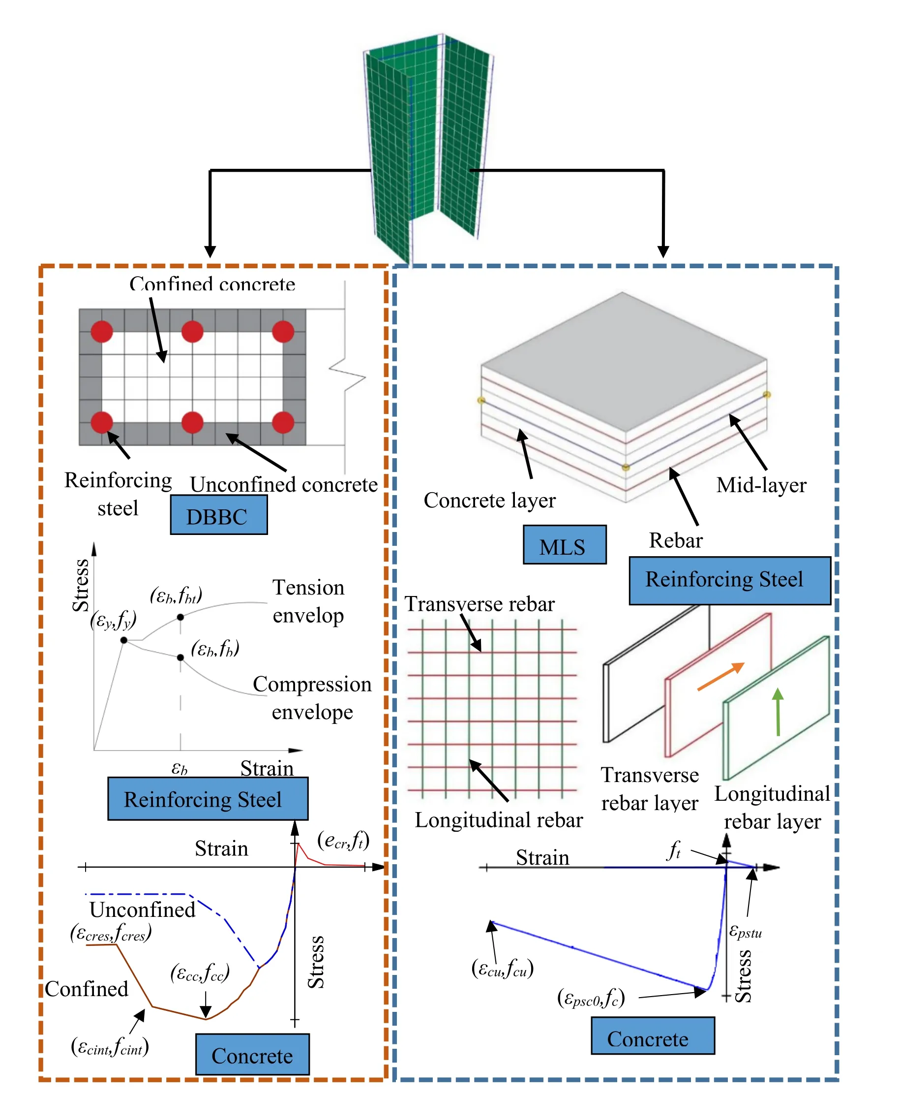
Figure 6:Modeling strategy for nonlinear RC structural wall response

Second,MLS elements are used to model the unconfined parts of the RC walls.This type of element is implemented in OpenSees as ShellNLDKGQ element [Lu,Tian,Cen et al.2017)].The element formulation includes plane membrane action and plate bending action with 6 degrees of freedom per each node.Finally,for deformation compatibility,rigid links are used to connect the MLS elements with the DBBC elements.There are three main practical reasons for using this approach,which are that it:(1) Improves the computational efficiency by eliminating the use of shell elements in the modeling of the boundary elements and corners of walls,(2) Allows for more flexible discretization of longitudinal reinforcing steel in fiber-sections of the DBBC element at boundary zones of RC walls,thus not limiting the discretization of bars to the mesh size of the MLS elements,(3) eliminates the need for regularization of the shell elements in confined regions,thus also limiting mesh size effects.

3.2 Material models

The uniaxial material “ConcretewBeta Material” [Lu and Panagiotou (2014)] implemented in OpenSees is used to model the unconfined and confined concrete regions of the fiber sections of the DBBC elements.The concrete model parameters shown in Fig.6 such as the confined concrete compressive stressfcc,strainεcc,and ultimate confined strainεcresare computed based on equations in Mander et al.[Mander,Priestley and Park (1988)].For the MLS element,a two-dimensional material model is used to simulate the nonlinear response of the unconfined concrete layers.The material model is an elasto-plastic damage model with smeared crack fixed orientation,in which cracks are assumed to form when the principal tensile stress exceeds the tensile strength of the concrete.After the formation of the cracks,the concrete material is treated as an orthotropic material instead of an isotropic one.The damage parameters in this model for tension behavior can be computed based on recommendations in Løland [Løland (1980)] while for the compression behavior,recommendations in Mazars [Mazars (1986)] are used.A shear retention factor (stc) is used after the formation of the cracks to reduce the shear modulus value and to simulate the interlocking behavior between the crack surfaces.Based on work of Rots et al.[Rots,Nauta,Kuster et al.(1985)],astcvalue ranging between 0.01 and 0.03 is used in this work.

The uniaxial material model that includes the buckling effects described previously is used to model the nonlinear response of the longitudinal reinforcing bars located at the boundary zones of the walls.The material model developed by Zsarnoczay [Zsarnoczay (2013)] is used as a base to simulate the cyclic response of reinforcing steel bars material model by adjusting the material parameters used in the original model implemented asSteel4in OpenSees.The proposed modifications by Monti et al.[Monti and Nuti (1992)] are used to account for buckling effects on the cyclic behavior of the steel material.The experimental results reported by Monti et al.[Monti and Nuti (1992)] are used to validate the cyclic model.A compression envelope curve for each specimen is developed separately using a reinforcing steel bar finite element model,which was developed to calibrate the Zsarnoczay [Zsarnoczay (2013)] material model parameters.Results in Fig.7 indicate that there is an excellent agreement between the cyclic predicted response and the experimental results for reinforcing steel bars with different slenderness ratios.In addition,the generic fatigue material developed by Uriz [Uriz (2005)],which was implemented in OpenSees as the uniaxialFatiguematerial is used to account for effects of low-cycle fatigue.The parameters for the fatigue material model are calibrated by using a recent set of experimental data presented in Barbosa et al.[Barbosa,Trejo,Nielson et al.(2017)].

For the MLS elements,smeared steel layers are defined with equivalent thickness to represent the physical location and direction of longitudinal and transverse reinforcing steel bars,where theSteel02uniaxial material model is used withPlateRebarmaterial to simulate the nonlinear response of the reinforcing steel bars in OpenSees.

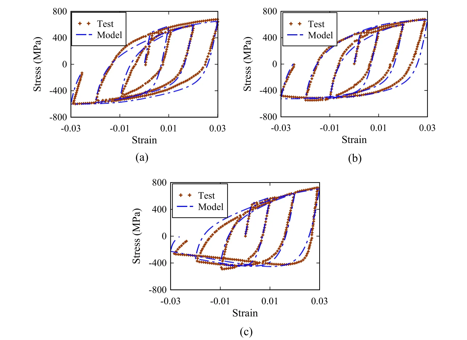
Figure 7:Validation of cyclic buckling model with experimental tests by Monti and Nuti (1992):(a) Specimen S5 L/D=5,(b) Specimen S8 L/D=8,and (c) Specimen S11 L/D=11

3.3 Regularization procedure

It is well known that nonlinear modeling of RC elements including softening response requires that a regularization procedure is needed.In this work,the regularization approach suggested by Coleman et al.[Coleman and Spacone (2001)] is used to regularize the response in compression softening.Thus,the regularizedεcuis given by:

whereGfcis the crushing energy of the concrete in compression,fc′ is the compressive strength of concrete,his the characteristic length of the element size,Ecis the concrete Young’s modulus,andεcois the compressive strain atfc′.

For a full-scale model of RC structural walls,the value ofGfcshould be selected carefully to ensure regularized predictions through nonlinear analysis,otherwise an overestimation of the drift capacity of an RC wall is obtained from the analysis when using higher values ofGfc.A parametric study is performed to evaluate the relationship betweenGfcand the nonlinear performance of two rectangular RC structural walls constructed entirely of unconfined concrete,which are specimens WR0 and WSH4 documented in Oh et al.[Oh,Han and Lee (2002)] and Dazio et al.[Dazio,Beyer and Bachmann (2009)],respectively.The WR0 specimen is a rectangular wall with 1.27% longitudinal steel ratio and unconfined boundary elements.The length of each boundary element is 13% of the total length of the wall.For the web zone of this wall,the horizontal reinforcement ratio is 0.28% and the vertical reinforcement ratio is 0.32%.The specimen has an axial load ratio of 10% and a shear span ratio equal to 2.The average concrete compressive strength for this specimen is 33 MPa at the day of testing.The WSH4 specimen is a rectangular wall with unconfined boundary zones,in which each boundary element is 10% of the total length of the wall with 1.54% longitudinal steel ratio,while the web part of the wall has a longitudinal reinforcement ratio of 0.54%.The transverse reinforcement ratio of the wall is 0.25%.The specimen has an axial load ratio of 5.7% and a shear span ratio equal to 2.28.The average concrete compressive strength for this specimen was 41 MPa at the day of testing.For the two specimens,the observed failure modes during the experiments are concrete crushing and bar buckling at the boundary elements.Using the modeling approach described previously for the unconfined parts of the walls,that is using MLS elements,three-dimensional FE models are developed in OpenSees.Following recommendations in Bazant [Bazant (1998)],the mesh size of 0.2 m×0.2 m is selected for the model discretization.A value forGfcranging between 35 and 100 N/mm is used to evaluate the simulated drift ratio (Dsim.) which are compared to the failure drift ratio from each test (Dtest).The results of the parametric study in terms ofGfcand obtained normalized drift ratios are shown in Fig.8.As it can be seen from the figure,a value of 82 N/mm ofGfcfor both walls is appropriate for the crushing energy of unconfined wall cross sections with the modeling parameters assigned.The data in Fig.8 indicate that using a normalized crushing energy equal to 2fc′ to 2.5fc′ can provide drift ratio predictions at most 4% off for both specimens.Naturally,these values are calibrated based on these test results,and future studies should further explore the values selected forGfc.The force-displacement and energy dissipation results for the tested walls using the forementioned value ofGfcare shown in Figs.9 and 10,respectively,and listed in Tab.4.As can be observed,the predicted initial stiffness,strength capacity,and ultimate displacement for both walls are in a good agreement with reported response from the tests.

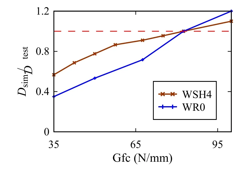
Figure 8:Simulated drift ratios using different crushing energy values for WR0 and WSH4 walls

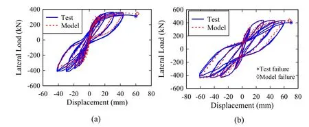
Figure 9:Force-displacement results from simulation and experimental data using of 82 N/mm (a) WR0 wall specimen (b) WSH4 wall specimen

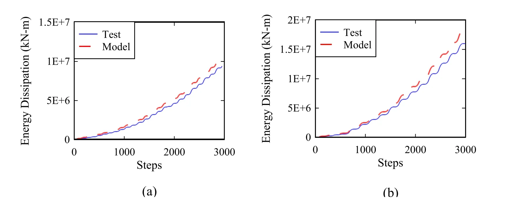
Figure 10:Energy dissipation results from simulation and experimental data using of 82 N/mm (a) WR0 wall specimen (b) WSH4 wall specimen

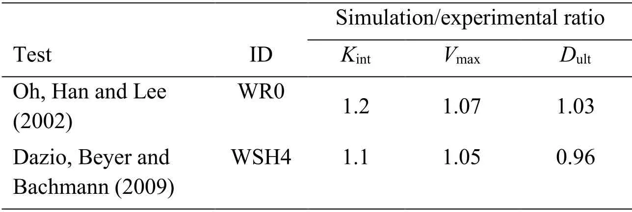
Table 4:Summary of simulation results using G fcvalue of 82 N/mm

4 Model validation

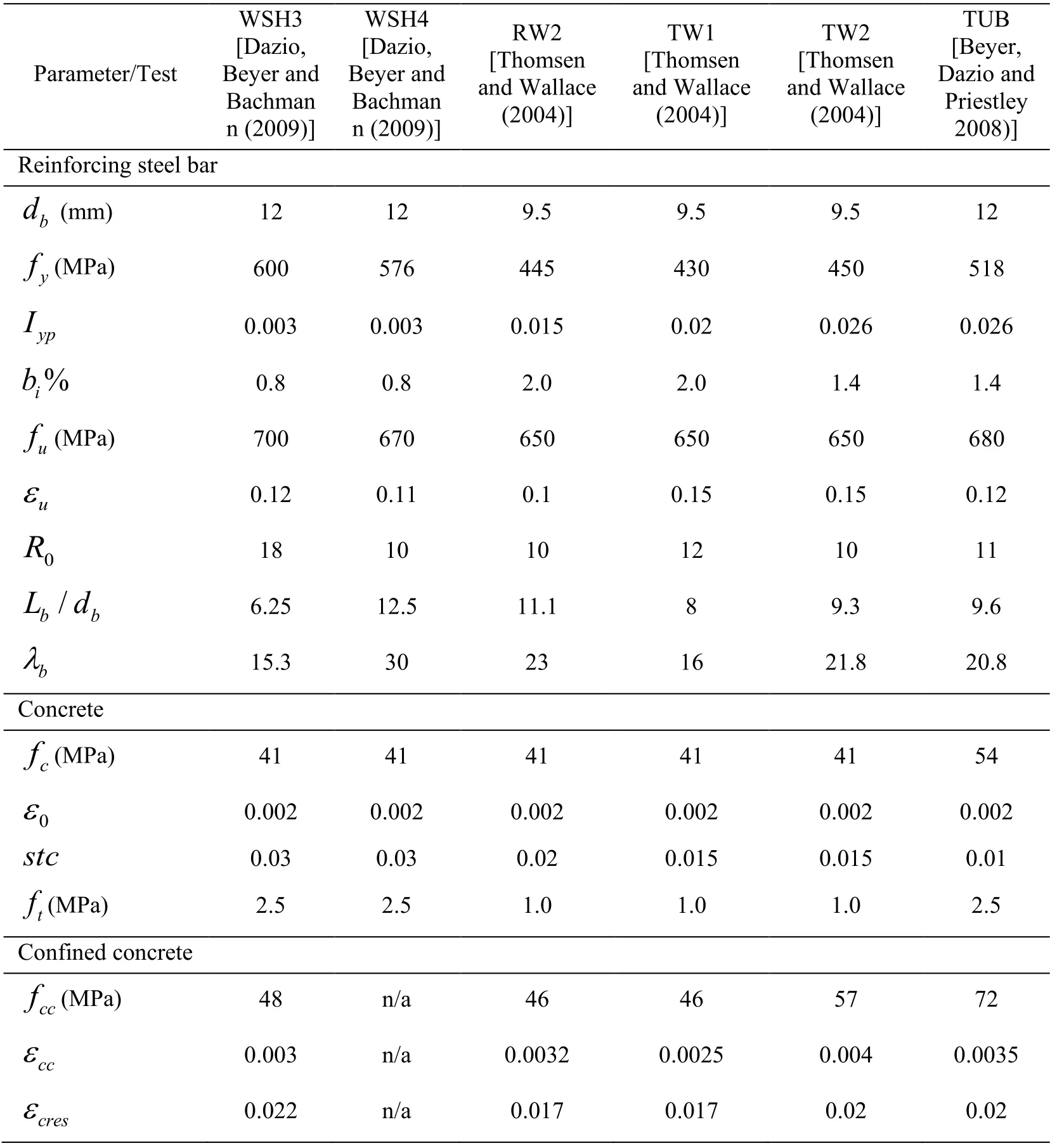
Six slender RC structural walls with different geometric shapes and various levels of confinement at the boundary elements are simulated using OpenSees with the developed numerical strategy described in the previous section of this paper.Tab.5 summarizes the general properties of the tested walls.For all case studies,the same value ofGfc.equal to 82 N/mm is used to regularize the concrete material models in compression.The predicted failure modes from the nonlinear analyses are compared with the experimental observations to evaluate the efficiency and versatility of the developed numerical strategy.Appendix C provides the parameters for the six tested structural walls that are used in the model validation.

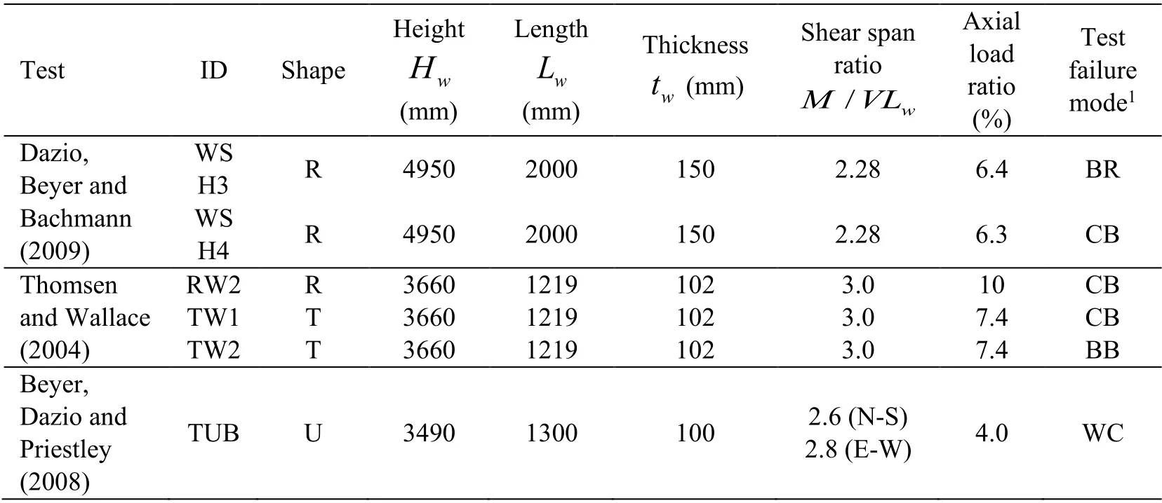
Table 5:Properties of six tested structural walls used for model validation

4.1 Specimens WSH3 and WSH4

The WSH3 and WSH4 specimens [Dazio,Beyer and Bachmann (2009)] correspond to rectangular cross-section (R-shape) RC walls (see Fig.11(b) and Fig.12(b)).The main testing design parameters are listed in Tab.5.Unlike specimen WSH3,specimen WSH4 had no confining or stabilizing reinforcing steel bars at the boundary elements.The tested units were fixed to reaction floor using post-tension bars.A horizontal displacement history was applied at the top of each wall by two hydraulic actuators.

During the testing,no early fracture of the longitudinal bars was observed for specimen WSH3.Additionally,at a drift ratio of 1.02%,spalling of the concrete cover initiated.The first sign of reinforcing steel bar buckling was observed at a drift ratio of 1.7%.One of the corner bars ruptured at a drift ratio of 1.8% because of bar buckling from the previous cycle.Similarly to specimen WSH3,the concrete spalling in specimen WSH4 initiated at a drift ratio of 1.02%.As the longitudinal reinforcing steel was not supported by any hoops or ties at the boundary zones,rebar buckling initiated immediately after the initiation concrete spalling,and thus the first bar buckling was observed at drift ratio of 1.02%.The buckling of the longitudinal reinforcing increased rapidly as the displacement demand of the test increased.At a drift ratio of 1.63%,for both specimens,concrete crushing at the boundary elements followed by reinforcing steel bar buckling of the exposed bars was the main mode of failure observed.

Figs.11(a) and Fig.12(a) show the developed numerical models for the WSH3 specimen and WSH4 specimen,respectively.The height of the wall is divided into twenty two equal lengths (0.2 m each) in which DBBC elements are used at the boundary zones and MLS elements used for the web with an element size of 0.2 m×0.2 m.Fig.11(c) and Fig.12(c) show the experimental response and the computed numerical response for WSH3 wall and

WSH4 wall,respectively.As can be seen from the figures,the computed response of each wall matches the obtained results adequately since the numerical models are able to predict the initial stiffness,the ultimate strength,and the peak drift ratio achieved.The computed peak lateral strength is 1.01 times the experimentally measured response for both RC walls.Moreover,the computed peak displacements are 1.3 and 1.1 times the experimentally measured response for WSH3 and WSH4,respectively.In addition,the numerical models predicted the observed mode of failure during testing which is mainly due to buckling of the reinforcing steel bars at the boundary element which lead to bar rupture of corner bars.Fig.11(d) and Fig.12(d) show the cumulative dissipated energy for the experiment and computed response for specimen WSH3 and WSH4,respectively.The cumulative dissipated energy errors at the end of the tests are 8.9% and 7.9% for WSH3 and WSH4,respectively.Fig.11(e) and Fig.12(e) illustrate the strain profiles from the experiment and the analysis along the height of the boundary element of the wall at drift ratios of 1.36% and 2.04% for the WSH3 wall,and at drift ratios of 0.68%,1.02%,and 1.36% for WSH4 wall.There is a good match between the measured strains and the predicted one especially up to a height of 0.5 m from the top of the foundation.However,the numerical models are not able to predict the nonlinear strain distribution for heights above 0.5 m for both RC walls,possibly due to unloading in the fiber sections of DBBC elements outside the predicted nonlinear plastic zone of the walls.Figs.11(f) and 12(f) show the strain profiles along the length of the WSH3 wall and WSH4 wall,respectively,at height of 0.2 m from the base as obtained from the analysis and test results.As can be seen,the proposed model is able to capture the nonlinear distribution of strain over the length of both walls reasonably well.However,possibly in part due to the fact that strain penetration is not modeled,the numerical models overestimate the predicted strain values at the wall ends for both loading directions.The computed maximum strains obtained from the analysis,at height of 0.2 m from the base,are 1.7 and 1.5 times the experimentally measured values for WSH3 wall at drift ratios of 1.36% and 2.04%,respectively.The computed maximum strains for WSH4 wall model are 1.9,1.5,and 1.3 times the experimentally measured values at drift ratios of 0.68%,1.02%,and 1.36%,respectively.

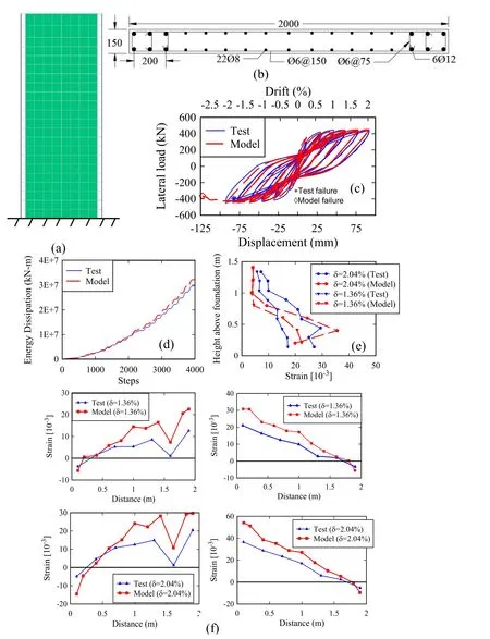
Figure 11:Case study 1 (WSH3) (a) developed numerical model (b) section reinforcing details,and test and model results for (c) force-displacement response (d) energy dissipation (e) strain distribution along the height of boundary element (f) strain distribution along the base of the RC wall at 0.2 m height

4.2 Specimen RW2

The RW2 specimen is a RC structural wall cyclic test with R-shape cross-section described in Thomsen and Wallace [Thomsen and Wallace (2004)] (Fig.13(b)).Tab.5 lists the main design characteristics of the test.During the testing,the first flexural reinforcement yielding occurred at the boundary element at a drift ratio of 0.75%,while concrete spalling was observed at a drift ratio of 1%.The lateral load capacity of the tested wall was maintained after two complete cycles were applied at drift ratio of 2.5%.The close spacing of hoops (5.33db) delayed the initiation of buckling of the reinforcement bars.At a drift ratio of 2.5% crushing at the boundary elements followed by reinforcing steel bar buckling of the exposed bars was observed during the test.All the eight longitudinal reinforcement bars buckled simultaneously at the boundary element for this wall.

Fig.13(a) shows the developed numerical model for the RW2 specimen.The height of the wall is divided into twenty four equal lengths (0.15 m each) in which DBBC elements are used at the boundary zones and MLS elements used for the web with an element size of 0.15 m×0.15 m.Fig.13(c) shows the experimental response with the computed numerical response.As can be seen from the figure,the computed response matches the obtained results adequately since the numerical model is able to predict the initial stiffness,the ultimate strength of the structural wall,and the maximum drift ratio.The computed peak lateral strength is 1.05 times the experimentally measured response,while the computed peak displacement is 1.04 times the experimentally measured response.In addition,the numerical model predicted the observed mode of failure which was mainly due to buckling of the reinforcing steel bars and concrete crushing at the boundary element.Fig.13(d) shows the cumulative dissipated energy for the experimental and computed response.The cumulative dissipated energy error at the end of the test is 6.2%.Fig.13(e) shows the strain profiles along the length of the wall at height of 0.15 m from the base that were obtained from the analysis and the test results.It should be noted that the strain profiles values for the tested RC wall were measured at an elevation of 0.2 m above the foundation.As can be seen,there is a satisfactory match with the results and the developed model is able to capture the nonlinear distribution of strain over the length and also the neutral axis location at a drift ratio of 2.0%.However,at a drift ratio of 1.0% there is a maximum error of 40% between the predicted strain and the value from the test.As the previous two RC walls,this difference in the obtained results is possibly due to the fact that strain penetration is not modeled.

4.3 Specimens TW1 and TW2

The TW1 and TW2 specimens are RC structural walls with T-shape section tested by Thomsen and Wallace [Thomsen and Wallace (2004)] (see Fig.14(b) and Fig.15(b)) under reversed cyclic loading in one direction.As described in Thomsen and Wallace (2004),the response of the TW1 specimen was affected by the direction of the applied loads (flange or web in tension or in compression).The lateral load capacity of the tested wall dropped rapidly when the applied displacement demand reached 45mm (at drift ratio of 1.25%) due to the poor detailing that was provided for the boundary element that was located at the web wall,furthest from the flange side.The large spacing between the transverse reinforcement contributed to the early buckling of the longitudinal reinforcement bars and the observed failure mode of this wall.

The nonlinear response of TW2 specimen was more ductile compared to TW1 wall,mainly due to the closer hoop spacing at the boundary element of the web.TW2 wall did not experience any loss in the lateral load capacity until the third cycle at drift ratio of 2.5%.The reported failure mode for this wall was an out-of-plane stability failure because of bucking of the reinforcing steel bars over several hoop spacings.

Figs.14(a) and Fig.15(a) show the developed numerical models for the TW1 specimen and TW2 specimen,respectively.The height of the wall is divided into eighteen equal lengths (0.2 m each) in which DBBC elements are used at the boundary zones and MLS elements used for the web with an element size of 0.2 m×0.2 m.Fig.14(c) and Fig.15(c) show the experimental response and the computed numerical response for both walls,respectively.As can be seen from the figures,the numerical model of each wall was able to simulate the ultimate strength of the tested structural wall and predict the peak drift ratio.The computed peak lateral strengths are 1.03 and 1.05 times the experimentally measured response for TW1 and TW2,respectively.Moreover,the computed peak displacements are 1.15 and 1.0 times the experimentally measured response for TW1 and TW2,respectively.Additionally,the numerical models predicted the observed mode of failure which was mainly due to buckling of the reinforcing steel bars at the boundary element that were located at web end opposite to the flange side.Moreover,concrete crushing also contributed to the overall dropping of the lateral capacity of the wall.Fig.14(d) and Fig.15(d) show the cumulative dissipated energy for the test and computed response of both walls.The cumulative dissipated energy errors at the end of the tests are 5.6% and 1.3% for TW1 and TW2,respectively.

Figs.14(e) and Fig.15(e) show the strain profiles along the flange of the wall at 0.2 m above the base that are obtained from the analysis and the test results.For the TW1 wall,the numerical model was able to predict the strain values accurately at the intersection between flange and web wall segments.However,the strain predicted underestimates the measured test values at the both ends of the flange wall segment.For the TW2,the numerical model was able to predict the strain values accurately along all length.Fig.14(f) shows the predicted strain profile along the web of the TW1 wall above 0.2 m from the base.The predicted strain profile was in excellent agreement with the measured values.

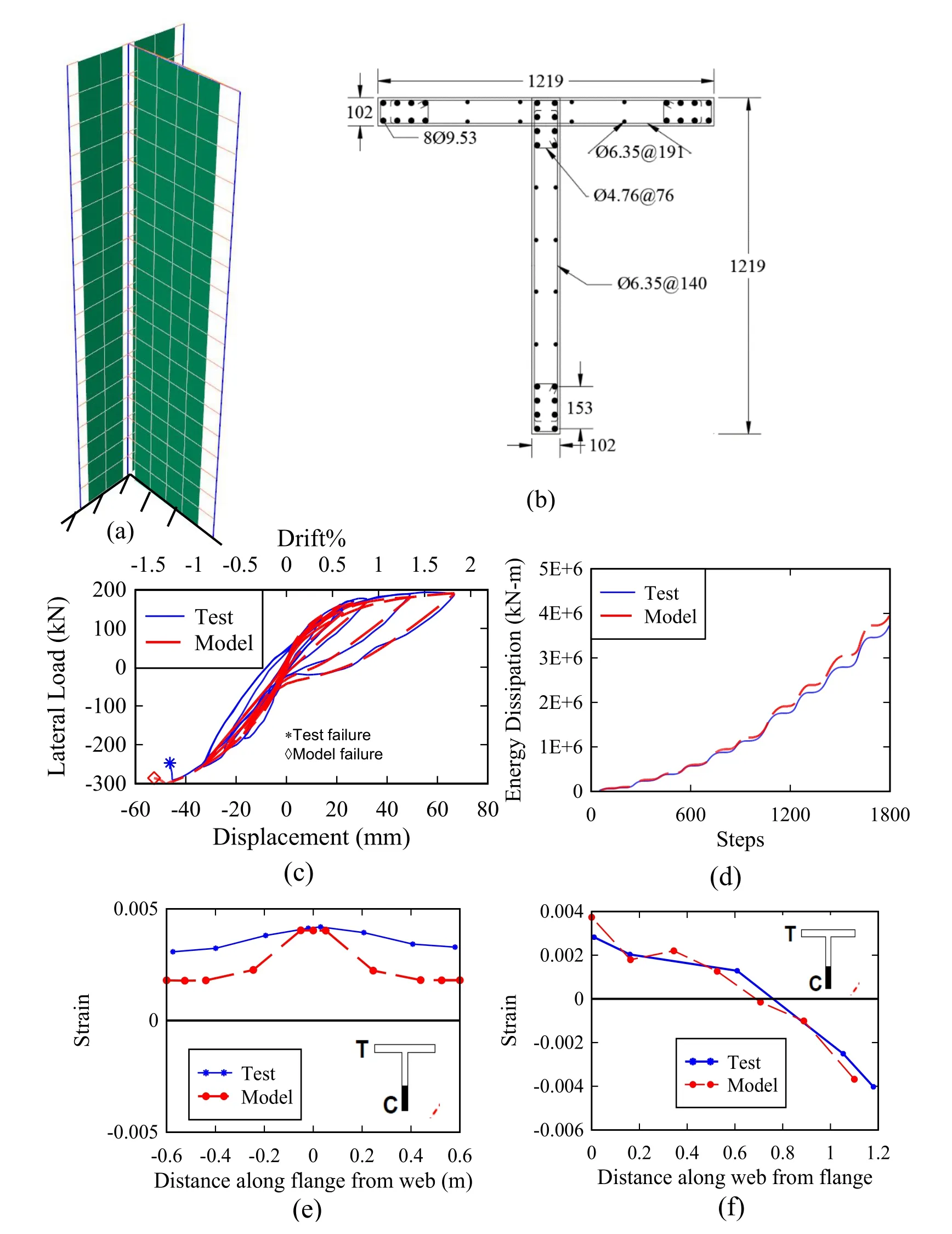
Figure 14:Case study 4 (TW1) (a) developed numerical model (b) section reinforcing details,and test and model results for (c) force-displacement response (d) energy dissipation (e) strain distribution along the flange segment of the RC wall at 0.2 m height (f) strain distribution along the web segment of the RC wall at 0.2 m height

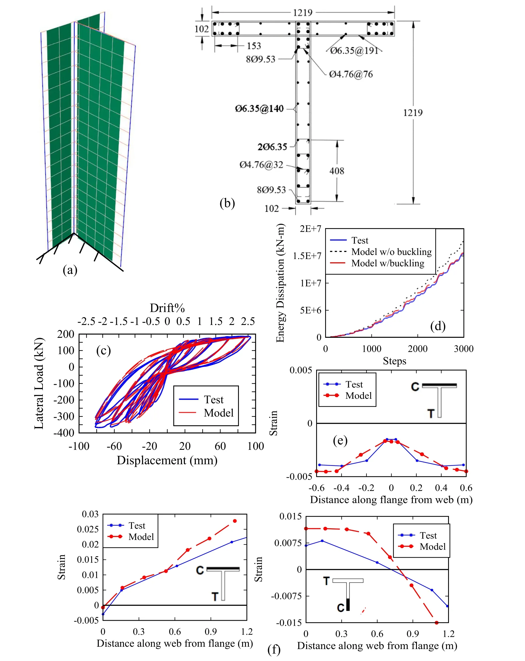
Figure 15:Case study 5 (TW2) (a) developed numerical model (b) section reinforcing details,and test and model results for (c) force-displacement response (d) energy dissipation (e) strain distribution along the flange segment of the RC wall at 0.2 m height (f) strain distribution along the web segment of the RC wall at 0.2 m height

Fig.15(f) shows the predicted strain profile along the web of the TW2 wall above 0.2 m from the base for two loading directions.The numerical model was able to predict the location of the neutral axis and the nonlinear distribution of the strain accurately.However,possibly due to not modeling the strain penetration,the numerical model underestimated the predicted strain values at one end of the wall for both loading directions.Morover,the effect of localization of the DBBC elements located at the boundary elements also contribute to this underestimation in the obtained strain values along the base of the walls.

4.4 Specimen TUB

The last example modeled is the TUB specimen described in Beyer et al.[Beyer,Dazio and Priestley (2008)].This case study corresponds to a U-shape section RC structural wall that was tested (Fig.16(b)) under reversed biaxial cyclic loading in two directions.Horizontal displacement histories were applied at the top of the wall by three hydraulic actuators.One actuator was used to load the web in E-W directions and two actuators were used to load the flanges in N-S direction.The E-W actuator located at height of 3.35 m while the N-S actuators located at height of 2.95 m.Four boundary elements were used in this specimen at the ends of each of the three wall parts.The wall was subjected to displacement cycles in each of the E-W,N-S,and diagonal directions as well as sweep cycles at each level of the applied displacement.The main failure mode reported from the test was crushing of compression diagonals in the unconfined part of the web.Even though this specimen did not exhibit failure due to bar buckling,this is considered to be a great example to validate the modeling approach developed.

Fig.16(a) shows the developed numerical model for the TUB specimen.The height of the wall is divided into twenty one equal lengths (0.15 m each) in which DBBC elements are used at the boundary zones and MLS elements used for the web with an element size of 0.15 m×0.15 m.Figs.16(c) and 16(d) show the force-displacement relation and the cumulative dissipated energy of the test results and computed numerical response in the NS direction,respectively.Figs.16(e) and 16(f) show the force-displacement relation and the cumulative dissipated energy of the test results and computed numerical response in the E-W direction,respectively.As can be seen from the figures,the numerical model was able to simulate the initial stiffness,ultimate strength,and the maximum drift ratio of the structural wall accurately.The computed peak lateral strengths are 0.9 and 1.02 times the experimentally measured values for N-S direction and E-W direction,respectively.Moreover,the computed peak displacements are 1.03 and 1.05 times the experimentally measured response for N-S direction and E-W direction,respectively.The cumulative dissipated energy errors at the end of the test are 10.4% and 2.5% for N-S direction and EW direction,respectively.It should be noted that for this case study there are no strain profiles provided by the test dataset to compare with.

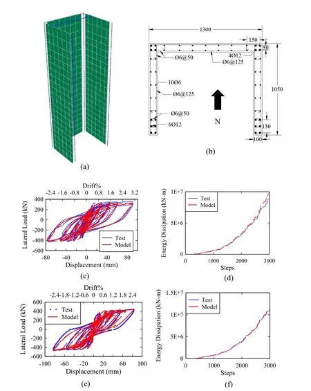
Figure 16:Case study 6 (TUB) ) (a) developed numerical model (b) section reinforcing details,and test and model results for (c) force-displacement response N-S direction (d) energy dissipation N-S direction (e) force-displacement response E-W direction (f) energy dissipation E-W direction

5 Discussion about the developed numerical strategy

Fig.17(a) shows the experimental response and the computed numerical response of specimen RW2 without including buckling effects of longitudinal reinforcing steel bars.The computed maximum difference in term of lateral strength is 1.1 times the experimentally measured response.There is an increase of 5% in terms of strength capacity when the buckling effects of reinforcing steel bars are not included.Additionally,the model was not able to predict the peak displacement at the failure point of the test.Fig.17(b) shows the cumulative dissipated energy for the experimental and numerical response.For the model without the buckling effects,the cumulative dissipated energy error at the end of the test is 14.6%.This value is larger than the obtained error of 6.2% when accounting for buckling effects of the reinforcing steel bars.

Fig.18(a) shows the experimental response with the computed numerical response of specimen TW2 without using buckling effects of longitudinal reinforcing steel bars.The computed maximum difference in term of lateral strength is 1.08 times the experimentally measured response.Similar to the obtained response of RW2 wall,there is an increase of 3% in terms of strength capacity when the buckling effects of reinforcing steel bars are not included with the numerical model.Additionally,the model was not able to predict the peak displacement at the test failure point.Fig.18(b) shows the cumulative dissipated energy for the experimental and numerical responses.For the model without the buckling effects,the cumulative dissipated energy error at the end of the test is 14.3%.This value is notably larger than the obtained error of 1.3% when accounting for buckling effects for the reinforcing steel bars.

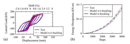
Figure 17:Obtained response of RW2 wall:(a) force-displacement response,and (b) energy dissipation

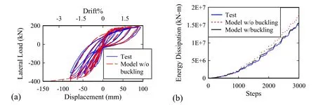
Figure 18:Obtained response of TW2 wall:(a) force-displacement response,and (b) energy dissipation

This section discusses the simulation results obtained from the numerical models using only multi-layered shell elements to simulate the nonlinear response of the structural walls.Figs.19(a) and 20(a) show the developed numerical models for the RW2 wall specimen by using two different shell element mesh sizes in the boundary elements of the wall.For the first model (mesh 1),a shell element size equal to the length of the boundary element is used.For the second model (mesh 2),each boundary element of the wall is subdivided into two shell elements in the direction of the cross-section of the wall.For models with mesh 1 and mesh 2,truss elements with uniaxial steel material are used to model the nonlinear response of the longitudinal reinforcing steel bars at the boundary elements of the wall.Figs.19(b) and 20(b) show the experimental response and the computed numerical response for RW2 wall of mesh 1 and mesh 2,respectively.As can be seen from the figures,both models overestimate the predicted lateral strength at drift ratios less than 1.5%,with maximum difference of 1.1 and 1.07 times the experimentally measured response for mesh 1 and mesh 2 models,respectively.Figs.19(d) and 20(d) show the computed responses by the models with displacement-based beam-column elements and models with only multi-layered shell elements for mesh 1 and mesh 2,respectively.As can be seen from the figures,the pinching effects are higher in the numerical models with only multi-layered shell elements.Figs.19(e) and 20(e) show the cumulative dissipated energy for the experimental and computed response.For the model with mesh 1,the cumulative dissipated energy error at the end of the test is 13.3%.For model with mesh 2,the cumulative dissipated energy error at the end of the test is 14.2%.These values compared with an obtained error of 6.2% when using displacement-based beam-column elements to model the boundary elements of the wall.

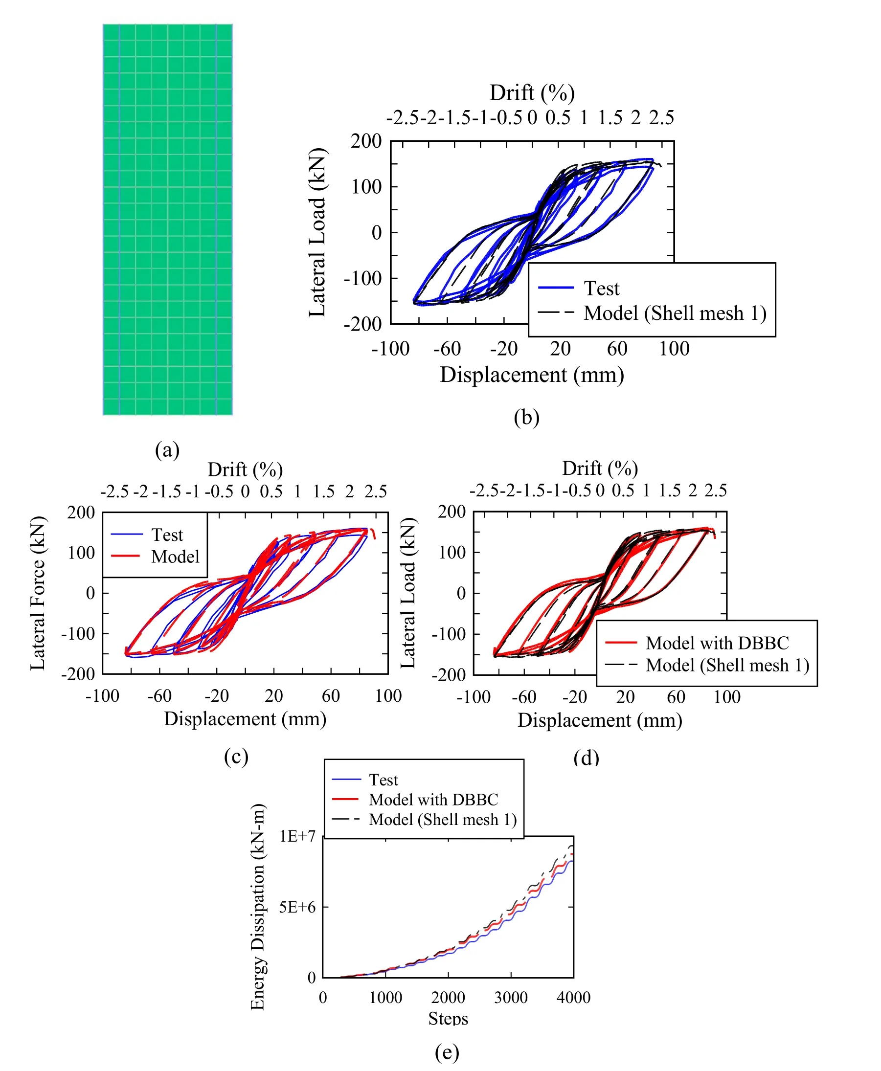
Figure 19:Specimen RW2 with mesh 1:(a) developed numerical model with mesh 1,(b) force-displacement response for model with mesh 1,(c) force-displacement response for model with DBBC elements,(d) force-displacement response for models with DBBC and MLS elements,and (e) energy dissipation

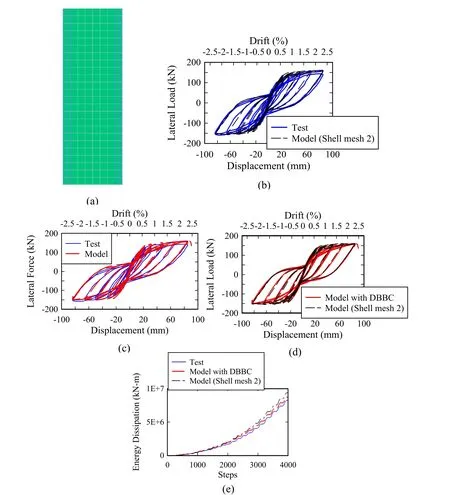
Figure 20:Specimen RW2 with mesh 2:(a) developed numerical model with mesh 2,(b) force-displacement response for model with mesh 2,(c) force-displacement response for model with DBBC elements,(d) force-displacement response for models with DBBC and MLS elements,and (e) energy dissipation

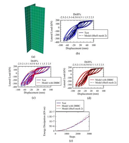
Figure 21:Specimen TW2:(a) developed numerical model,(b) force-displacement response for model with MLS elements,(c) force-displacement response for model with DBBC elements,(d) force-displacement response for models with DBBC and MLS elements,and (e) energy dissipation

Fig.21(a) shows the developed numerical model for the TW2 wall specimen by using only multi-layered shell elements to model the nonlinear response of the wall.A similar modeling approach to the one described in the RW2 case was used when using layered shell elements for modeling the boundary elements.Fig.21(b) shows the experimental response and the computed numerical response for TW2 wall.As can be seen from the figure,the numerical model was able to predict the cyclic response of the wall with computed peak lateral strength of 0.92 times the experimentally measured response when the flange of the wall was under compression load.However,the numerical model underestimates the initial stiffness and was not able to simulate the nonlinear response of the wall accurately at higher drift demands when compression load was applied on the web of the wall.It should be noted that the obtained nonlinear response when compression load is applied on the web of the wall can be improved by increasing the concrete tension strength of the unconfined parts of the wall.However,this also would lead to overestimation of the response of the wall when the flange of the wall is under compression.Fig.21(d) compares the computed response obtained from the model with displacementbased beam-column elements and the model with only multi-layered shell elements.As can be seen from the figure,the pinching effects are higher in the numerical model with only multi-layered shell elements.Fig.21(e) shows the cumulative dissipated energy for the experimental and computed response.For the model that built entirely with multilayered shell elements,the calculated cumulative dissipated energy error at the end of the test is 17%.This value is considerably larger than the obtained error of 1.3% when using displacement-based beam-column elements to model the boundary elements of the wall.

6 Conclusion

This paper presented the development of an analytical model to predict the buckling length of reinforcing steel bars embedded in RC elements and a FE modeling strategy to simulate the nonlinear response of slender RC structural walls with different geometrical sections.Models developed were implemented in OpenSees.

In the first part of the paper,parameters of a uniaxial material model (Steel4) of reinforcing steel bar including buckling effects are adjusted based on the proposed buckling length model in this study.Five experimental specimens of structural wall boundary elements with different level of confinement are used to validate the developed analytical model.

In the second part of this paper,multi-layer shell elements and displacement-based beamcolumn fiber-section elements are combined to model the web and boundary elements parts of RC structural walls,respectively.This modeling approach improves the computational efficiency when compared to using only multi-layer shell elements and allows for more flexible discretization of longitudinal reinforcing steel bars in the fiber sections located at the boundary elements.A regularization procedure is carried out to eliminate the mesh size effects for multi-layer shell elements on the obtained results from the nonlinear analyses.Finally,to validate the developed numerical tool,six slender RC structural walls with Rshape,T-shape,and U-shape section,and various level of confinement at the boundary elements,are used as case studies.The predicted responses by the modeling approach are in a good agreement with the reported results from the experimental measurements for all specimens.Moreover,the proposed model is able to simulate the nonlinear response of specimens with different failure modes.Particularly,the flexural degradation response due to concrete crushing and buckling of the reinforcing steel bars at the boundary elements is captured by the developed model.In addition,there is a reasonably good agreement between the obtained strain profiles from the analysis with the experimental strain measurements for all specimens.However,the strain penetration effects of the longitudinal reinforcement are not included in the modeling approach developed and differences were observed at strains at the base of the walls.In future studies,including strain penetration effects in the modeling would potentially improve the predicted local response along the base length of the structural wall.

In this study,the regularization procedures for the unconfined part of the structural walls are based on the experimental results of only two rectangular structural walls due to the limited available data in the literature.There is a need to develop an experimental program to study in more depth the effects of concrete strength on the concrete crushing energy for rectangular and non-rectangular structural walls and to develop a set of benchmark tests that can be used for verification and validation of future wall modeling efforts.

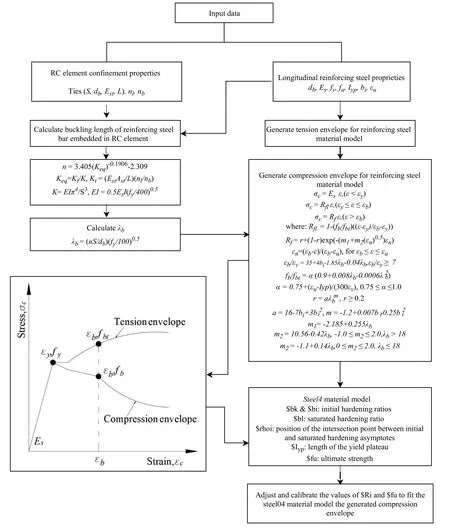
Appendix A:Reinforcing steel bar buckling compression enevelope and length.

Appendix B:Application to calculate embedded reinforcing steel bar buckling compression envelope and length

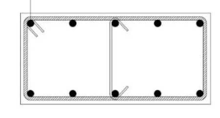
Taleb et al.[Taleb,Tani and Kono (2016)] specimen ID 4

Input parameters:

Longitudinal bar:

E s ( MPa) f y ( MPa) I yp b i % fu ( MPa) εu d b( m m) 200,000 347 0.0 0.8 500 0.1 10

Transverse bar:db= 4mm,S= 80mm,Es=200,000MPa

Calculate the buckling length of embedded reinforcing steel bar

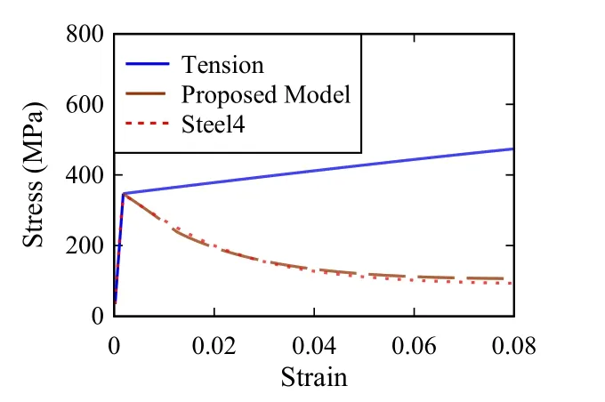
Generate the compression envelope for reinforcing steel material model

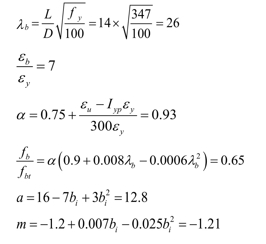
Parameters forSteel4material model (compression model)

-Kin apply kinematic hardening

$bk:0.001 (hardening ratio)

$Rb0:8.0,$r1:0.91,$r2:0.15

-iso apply isotropic hardening

$bi:-0.048 (initial hardening ratio)

$bl:0.0000002 (saturated hardening ratio)

$rhoi:-0.83 (specifies the position of the intersection point between initial and saturated hardening asymptotes)

$Ri:2.0 (control the exponential transition from initial to saturated asymptote)

$Iyp:0.0 (length of the yield plateau)

-ult apply an ultimate strength limit

$fu:347 (MPa) (ultimate strength)

$ Ru:5.0 (control the exponential transition from kinematic hardening to perfectly plastic asymptote)

Appendix C:Parameters for the six tested structural walls that used for model validation

Parameter/Test BBn[We aD(yc2 ae Sh0 zr Hm0 ia9 o3an),n d] BBn[e W aD(yc2 Saeh0 zr Hm0 iao9 4an,) n d] a[nTd(2 hR W0 oW0ma4 2ls)l ea] nc e an[T d(2 hT W0 oW0ma4 1ls)l ea] nc e a[nTd(2 hT W0 oW0ma4 2ls)l ea] nc e D P[a2rB Tzi0eeiU0osy8t B ela)er ]n,y d Reinforcing steel bar d b (mm) 12 12 9.5 9.5 9.5 12 fy(MPa) 600 576 445 430 450 518 I yp 0.003 0.003 0.015 0.02 0.026 0.026 bi % 0.8 0.8 2.0 2.0 1.4 1.4 fu(MPa) 700 670 650 650 650 680 εu 0.12 0.11 0.1 0.15 0.15 0.12 R0 18 10 10 12 10 11 Lb /d b 6.25 12.5 11.1 8 9.3 9.6 λb 15.3 30 23 16 21.8 20.8 Concrete fc(MPa) 41 41 41 41 41 54 ε0 0.002 0.002 0.002 0.002 0.002 0.002 stc 0.03 0.03 0.02 0.015 0.015 0.01 ft(MPa) 2.5 2.5 1.0 1.0 1.0 2.5 Confined concrete f cc(MPa) 48 n/a 46 46 57 72 εcc 0.003 n/a 0.0032 0.0025 0.004 0.0035 εcr es 0.022 n/a 0.017 0.017 0.02 0.02