RAIM Algorithm Based on Fuzzy Clustering Analysis
Shouzhou Gu , Jinzhong Bei Chuang Shi, Yaming Dang Zuoya Zheng and Congcong Cui
Abstract: With the development of various navigation systems (such as GLONASS, Galileo, BDS), there is a sharp increase in the number of visible satellites.Accordingly, the probability of multiply gross measurements will increase.However, the conventional RAIM methods are difficult to meet the demands of the navigation system.In order to solve the problem of checking and identify multiple gross errors of receiver autonomous integrity monitoring (RAIM), this paper designed full matrix of single point positioning by QR decomposition, and proposed a new RAIM algorithm based on fuzzy clustering analysis with fuzzy c-means (FCM).And on the condition of single or two gross errors, the performance of hard or fuzzy clustering analysis were compared.As the results of the experiments, the fuzzy clustering method based on FCM principle could detect multiple gross error effectively, also achieved the quality control of single point positioning and ensured better reliability results.
Keywords: Integrity, RAIM, FCM, single point positioning.
1 Introduction
Surveying and navigation industries have been revolutionized over the past three decades by the global navigation satellite system (GNSS).The integrity of GNSS is a major limitation for many existing and potential applications.GNSS integrity refers to the ability of the system to alert users when the navigation system fails or the positioning cannot be used for navigation and positioning [Bei (2010)].As a measure of the user's availability of information provided by the system and an important parameter, receiver autonomous integrity monitoring (RAIM) refers to monitoring the completeness of user positioning results based on redundant observations from the user receiver.RAIM is a key part in the integrity monitoring system and the last link to ensure the security of user positioning [Parkinson, Spilker, Axelrad et al.(1996)].
The RAIM algorithms have always become research focuses in the GNSS field.RAIM is the ability to detect and identify the failures in GNSS by using measurements from receiver which needs more than 4 visible satellites to detect failures and more than 5 to identify.
The current RAIM algorithms, mainly including the parity vector method [Wang, Zhang, Xu et al.(2016); Li and Li (2012)], the least squares residual method [Li, Zhu, Yang et al.(2016)], and the approximate radial error protection method [Hunzinger, Morgren, Studenny et al.(1997)], use the residual comparison to perform fault detection, which has a better recognition effect for a single gross error, but has a poor effect under multiple gross errors.The overall least squares method [Juang (2000); Jeon and Lachapelle (2005); Yang, Liu and Zhang (2009)] can perform fault detection and fault identification, but because it takes into account the correspondence between the smallest singular value mutation and the satellite fault, the algorithm is complex, the calculation load is heavy, and the timeliness is not satisfied; In addition, the maximum de-separation method [Nowak (2015); Joerger, Chan and Pervan (2014)], the weighted RAIM method [Yu (2008)], the Bayesian method [Zhang and Gui (2015)] and the Kalman filter algorithm [Song, Hou and Xue (2017)] have not solved the fault identification problem well.
With the development of various navigation systems (such as GLONASS, Galileo, BDS), there is a sharp increase in the number of visible satellites.Accordingly, the probability of multiply gross measurements will increase.However, the conventional RAIM methods are difficult to meet the demands of the navigation system.In order to solve this problem, this paper proposes a new RAIM algorithm based on fuzzy clustering analysis, which can effectively solve the problem of detection and recognition of multiple gross errors.
2 Principle of fuzzy clustering analysis
Fuzzy clustering analysis is a mathematical method that uses fuzzy mathematics to describe and classify things according to certain requirements.Fuzzy clustering analysis generally refers to constructing a fuzzy matrix according to the attributes of the concerned object itself.The clustering relationship is determined according to a certain degree of membership, that is, fuzzy mathematics is used to quantitatively determine the fuzzy relationship between samples to objectively and accurately cluster.There are many clustering methods, such as based on similarity relations and fuzzy relations, transitive closures based on fuzzy equivalence relations, maximum support trees based on fuzzy graph theory, and methods based on convex decomposition, dynamic programming and difficult identification of data.But the most widely used in practice is the fuzzy clustering method based on objective function.This paper selects the most complete and widely used fuzzy c-means (FCM) based on the objective function-based clustering algorithm.
A given data set X={x1,x2,…,xn} is a set of finite set of observation samples for n modes in the pattern space, xk={xk1,xk2,…,xks} is the eigenvector of the observed sample xk, corresponding to a point of the feature space.xkjis the assignment on the j-th dimension of the feature vector xk.For a given sample X, if it is divided into class c, then corresponding to c class centers.Each sample belongs to a class i with a membership degree of uij.Then define an FCM objective function and its constraints are as follows:

where


where, m is called a weighted exponent or smoothing parameter and is a membership factor; dijrepresents the degree of distortion between the sample xjin the i-th class and the i-th cluster center ci, measured by the distance between the two vectors.As shown in Eq.(4).

The criterion for clustering is to take the minimum value of the objective function, that is:

We can obtain

Furthermore, we have

It can be known from the constraint condition 2 expressed in Eq.(3)

that

As can be seen from the above, if the data set X, the clustering class number c, and the weight m are known, the best fuzzy classification matrix and cluster center can be determined from the above equation.
3 Construction of full design matrix
3.1 Definition of full design matrix
In the single-point positioning based on the least squares, the observational equation reads,

where “l ” represents the pseudo-range residuals, l=ρ-Dis-δ0

B is the coefficient matrix, XSi=(xsi,ysi,zsi) represents the position of satellite i, X=(x,y,z) represents the position of user, δx=(dx,dy,dz,dt) is the user’s position and time bias, ρ is the pseudo-range, δ0is the sum of various error including troposphere and ionosphere error, which is calculated by model, Disiis the distance of user and the satellite i, n is the number of satellite.
Then the user location can be given by the LS estimation

At the same time, we can obtain the reliability matrix R, it is expressed an equation (17).

Where I is the n-dimensional unit matrix
The properties of the reliability matrix R include
(1) The reliability matrix R is an idempotent matrix, it means R2=R.
(2) The reliability matrix R is not full rank matrix, its rank is n-t, n is the number of satellite and t is necessary observation number, in here t=4.
Suppose there is a linear transformation, it is expressed as equation (18)

Then, we can obtain the definition of QR parity check vector t,

The properties of the QR parity check vector t are as follows

QR parity check vector conversion matrix T is a special transformation that transforms ndimensional observation space into n-4 dimensional parity space.T has the following special properties:
(1) Each row of T is orthogonal to the columns of B;
(2) The rows of T are orthogonal to each other;
(3) The rows of T are normalized, and the size of each row is unity;
In the QR parity method, it is proved that:

Eq.(19) is defined by the QR parity check vector, and l is replaced by its equivalent Bδx-V.Since the orthogonal propertyTB=0, and we have:

Where: t is the QR parity detection vector; T is the QR parity detection generation matrix; ε is the negative residual.
The matrix expansion can be obtained from Eq.(23):

where: m=n-4;n is the number of satellites; εi(i=1,2,…,n) is the negative residual of observation i, which is a numerical variable.

Where Tiis the columns i of T determined by the geometric matrix of the satellite position, εiis determined by the functional characteristics of the observation, so εiTiis determined by the observation error and the satellite geometry matrix.When there is a gross error in a certain measurement, it will be expressed that the ‖ εiTi‖ value of the observation is larger, that is, the modulus of the vector εiTiis larger; and it has an advantage in the left half of the formula (25) medium, that is, the share is relatively large.Therefore, the formula (25) the right part of the middle part is mainly affected by the gross error εiT, so the QR parity check vector t has a relatively strong correlation with the influence vector εiPiof the error observation.
By converting the formula (25) into a matrix form, you can get:

That is, the left part and the right part in the formula (26) are combined, and this formula is called a full design matrix.
3.2 Calculation of full design matrix
The full design matrix is calculated by coefficient matrix Bn×4.Firstly, we take QR decomposition for matrix Bn×4.

The QR decomposition (also called the QR factorization) of a matrix is a decomposition of the matrix into an orthogonal matrix and a triangular matrix.A QR decomposition of a real square matrix B is a decomposition of B as B = QS, where Q is an orthogonal matrix and S is an upper triangular matrix.If A is nonsingular, then this factorization is unique.It means that

The upper triangular matrix can be express asis 4×4 an upper triangular matrix, Syis a (n-4)×4 zero matrix.
Similarly, we can take the transpose of orthogonal matrix Q asis 4×n matrix, Qyis a (n-4)×n matrix.
Then, for the observational equation V=Bδx-l, we can know

Eq.(29) are multiplied by the transpose of orthogonal matrix Q on both sides.

then

Because Syis a (n-4)×4 zero matrix, we can know

If we take Qyl=QyV=t, then Qyis the full design matrix.
4 Single-point positioning RAIM algorithm based on FCM
The full design matrix in Section 3 of this paper is a sample of fuzzy clustering.Each column of the full design matrix represents a satellite.The specific clustering process is as follows:
(1) Calculate the relative distance matrix D of the full design matrix.

(2) The number of clustering categories is determined.This paper determines three categories, which are health observations, suspected outliers and outliers.The maximum, minimum and intermediate values are selected as cluster centers.
(3) Calculating the membership function

(4) Update cluster center

(5) Calculating the variation of cluster centers

(6) If Δ is less than the threshold, stop the calculation, otherwise repeat Step 3 to Step 5.
5 Experiments and analysis
5.1 Data and experimental scheme
Method availability analysis uses two options:
(1) Introducing a single gross error (introducing a 4 m magnitude gross error on a single value of negative residual ε), performing gross error detection and identification, and comparing it with hard cluster analysis.
(2) Introducing two gross errors (introducing the 4 m magnitude gross error on the two values of the negative residual ε), performing gross error detection and identification, and comparing with the hard cluster analysis.
The data is based on the data in [Bei (2010)].C001 station in the continuous operating reference stations (CORS) network in Hebei Province.The data time is UTC 0:00:00-24:00:00 on August 1, 2017.The data sampling rate is 30 s.
5.2 Introducing a single gross error
This study selects an observation epoch of the C001 station.According to the single-point positioning model, there are 4 unknowns, including the coordinates XYZ of the position to be fixed and the receiver clock error t.The basic observation equation is n×4, then QR parity check method produces matrix T is (n-4)×4.In this example, the number of satellites is n=9.This example starts with the matrix T and matrix ε obtained after QR decomposition.
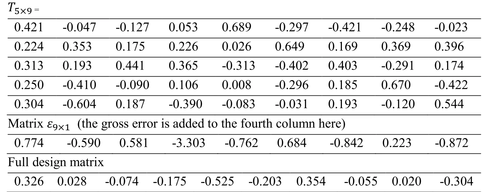
T5×9 = 0.421 -0.047 -0.127 0.053 0.689 -0.297 -0.421 -0.248 -0.023 0.224 0.353 0.175 0.226 0.026 0.649 0.169 0.369 0.396 0.313 0.193 0.441 0.365 -0.313 -0.402 0.403 -0.291 0.174 0.250 -0.410 -0.090 0.106 0.008 -0.296 0.185 0.670 -0.422 0.304 -0.604 0.187 -0.390 -0.083 -0.031 0.193 -0.120 0.544 Matrix ε9×1 (the gross error is added to the fourth column here) 0.774 -0.590 0.581 -3.303 -0.762 0.684 -0.842 0.223 -0.872 Full design matrix 0.326 0.028 -0.074 -0.175 -0.525 -0.203 0.354 -0.055 0.020 -0.304
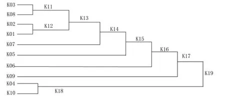
Figure 1: Cluster graph of one single gross error with hard cluster analysis methods

0.173 0.208 -0.102 -0.746 -0.020 0.444 -0.142 -0.082 0.345 0.078 0.242 -0.114 -0.256 -1.206 0.239 -0.275 -0.339 -0.065 -0.152 -1.926 0.193 0.242 -0.052 -0.350 -0.006 -0.202 -0.156 0.149 0.368 0.186 0.235 0.356 0.109 1.288 0.063 -0.021 -0.163 -0.027 -0.474 1.367
5.2.1 Using hard clustering analysis
Calculate the correlation distance matrix by using the Mahala Nobis distance calculation method according to the full design matrix:
Further cluster analysis is shown in Fig.1.
As can be seen from Fig.1, the class 10 and class 4 are finally synthesized into one class, because class 10 is a gross error class, it is classified as a gross error class; Other classes fall into one category, which is a random error class.Obviously, the gross error is separated.
5.2.2 Using fuzzy class analysis
According to the full design matrix, the Mahala nobis distance calculation method is used to calculate the correlation distance matrix, and three initial cluster centers are set.According to the distance as the initial membership coefficient, and then iterative operation, and finally all the data into three categories, the clustering results shown in Fig.2.
As can be seen from Fig.2, all classes are finally divided into three categories: the first class contains class 1, class 2, and class 9; the second class contains class 10 and class 4; and the third class contains class 3, class 5, class 6 and class 7.Where class 10 is a known gross error class, so the second class is a gross error class; There are large correlations between multiple subclasses (class 5, class 6, class 7, class 9) in the first class and the third class, so they are grouped into one class called health class.
It can be seen from Fig.1 and Fig.2 that the hard cluster analysis method and the fuzzy clustering analysis method can better realize the gross error recognition under the condition of single gross error.
5.3 Introducing two gross errors
This study selects the same observation epoch from the introduction of a single gross error.According to the single-point positioning model, there are 4 unknowns, including the coordinates XYZ of the position to be fixed and the receiver clock error t.The basic observation equation is n×4, then QR parity check method produces matrix Tis (n-4)×4.In this example, the number of satellites is (n=9.This example starts with the matrix Tand matrix ε obtained after QR decomposition.
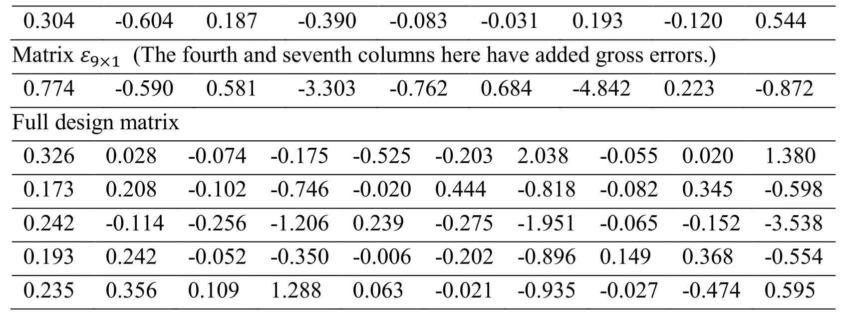
0.304 -0.604 0.187 -0.390 -0.083 -0.031 0.193 -0.120 0.544 Matrix ε9×1 (The fourth and seventh columns here have added gross errors.) 0.774 -0.590 0.581 -3.303 -0.762 0.684 -4.842 0.223 -0.872 Full design matrix 0.326 0.028 -0.074 -0.175 -0.525 -0.203 2.038 -0.055 0.020 1.380 0.173 0.208 -0.102 -0.746 -0.020 0.444 -0.818 -0.082 0.345 -0.598 0.242 -0.114 -0.256 -1.206 0.239 -0.275 -1.951 -0.065 -0.152 -3.538 0.193 0.242 -0.052 -0.350 -0.006 -0.202 -0.896 0.149 0.368 -0.554 0.235 0.356 0.109 1.288 0.063 -0.021 -0.935 -0.027 -0.474 0.595
5.3.1 Using hard clustering analysis
Calculate the correlation distance matrix by using the Mahala nobis distance calculation method according to the full design matrix:
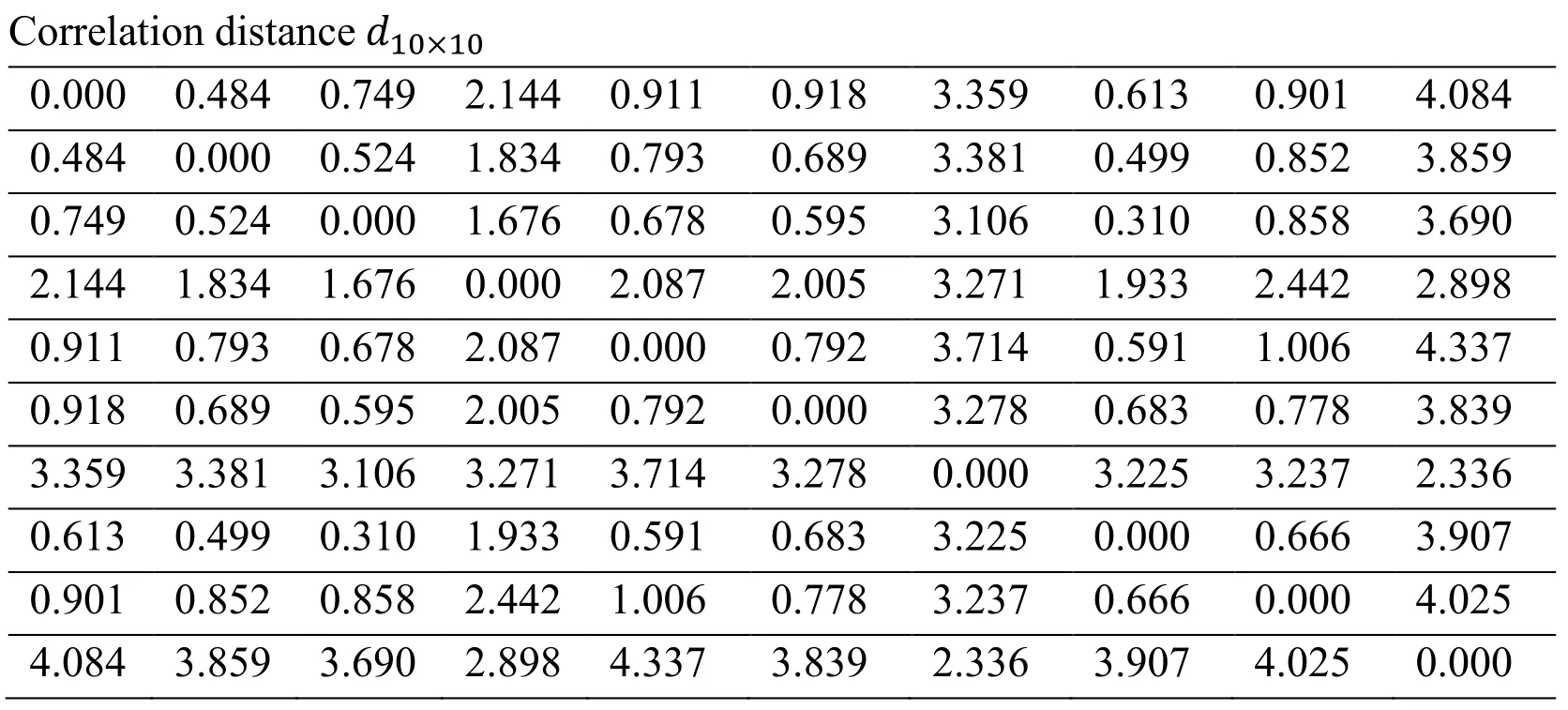
?
Cluster analysis is shown in Fig.3.
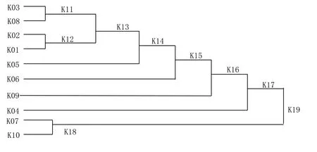
Figure 3: Cluster graph of two gross errors with hard cluster analysis methods
As can be seen from Fig.3, class 10 and class 7 are finally synthesized into one class, which is classified as a gross error class; Other classes fall into one category, which is a random error class.Obviously, the largest gross error that existed was first separated, but the gross error class 4 was not identified.
5.3.2 Using fuzzy class analysis
According to the full design matrix, the Mahala nobis distance calculation method is used to calculate the correlation distance matrix, and three initial cluster centers are set.According to the distance as the initial membership coefficient, and then iterative operation, and finally all the data into three categories, the clustering results shown in Fig.4.
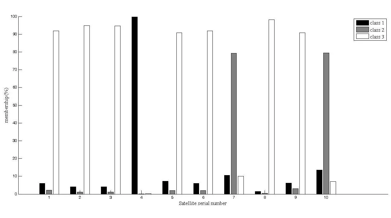
Figure 4: Membership Map of Two Gross Errors with Fuzzy Cluster
As can be seen from Fig.4, all classes are finally divided into three categories: the first class contains class 4; the second class contains class 10 and class 7; and the third class contains class 1, class 2, class 3, class 5, class 6, class 7 and class 9.Where class 10 is a known gross error class, so the second class is a gross error class.As can be seen from Fig.4, the first class has only one single sample, which is the isolated data, which can be judged as gross error data, which is classified as gross error class; the remaining the third class is classified as health class.
It can be seen from Fig.3 and Fig.4 that the fuzzy clustering analysis method effectively realizes the gross error recognition under the condition of two gross errors, but the hard cluster analysis method recognizes at one time.
5 Citations
With the development of various navigation systems (such as GLONASS, Galileo, BDS), there is a sharp increase in the number of visible satellites.Accordingly, the probability of multiply gross measurements will increase.However, the conventional RAIM methods are difficult to meet the demands of the navigation system.Aiming at the identification problem of multiple gross errors in GNSS RAIM, this paper introduces the fuzzy clustering analysis method of FCM, and then the full design matrix of single point positioning constructed by QR parity check method is taken as the initial sample.and studies the RAIM method based on fuzzy clustering analysis method.Combined with the actual observation data, it is compared with the traditional cluster analysis method.It can be seen from the results that the method can effectively realize the identification of multiple gross errors, and has certain application value for gross error recognition in practical engineering.
Acknowledgement:This work was supported by “Key Project of China National Programs for Research and Development (No.2016YFB0501801, No.2016YFB0502105, No.2016YFB0501405), International GNSS Monitoring & Assessment System (iGMAS, No.GFZX0301040308-06), Fundamental Research Funds of the CASM(AR1901), The National High-tech Research and Development Program of China (863 Program) (No.2015AA124001), The Fundamental Research Funds for CASM(No.7771730) and thanks for the data from Hebei province surveying and mapping data archives.
References
Bei, J.Z.(2010): GNSS Integrity Monitoring Method, Technology and Application.Wuhan: Wuhan University.
Bei, J.Z.(2012): Theory and Application of GNSS Integrity Monitoring.Beijing: Surveying and Mapping Press.
Hunzinger, J.F.; Morgren, S.D.; Studenny, J.(1997):CDGPS RAIM algorithm and protection radius calculation.Proceedings of International Technical Meeting of the Satellite Division of the Institute of Navigation.
Jeon, C.W.; Lachapelle, G.(2005): A new TLS-based sequential algorithm to identify two failed satellites.International Journal of Control, Automation, and Systems, vol.3, no.2, pp.166-172.
Joerger, M.; Chan, F.C.; Pervan, B.(2014): Solution separation versus residual-based RAIM.Navigation, vol.61, no.4, pp.273-291.
Juang, J.C.(2000): On GPS position and integrity monitoring.IEEE Transactions on Aerospace and Electronic Systems, vol.36, no.1, pp.327-336.
Li, C.; Zhu, L.F.; Yang, Q.(2016): Research on receiver autonomous integrity monitoring by least squares residuals.GNSS World of China, vol.41, no.1, pp.69-72.
Li, Y.; Li, M.(2012): Study on RAIM algorithm of GPS receiver based on parity vector.Geomatics & Spatial Information Technology, vol.35, no.1, pp.158-160.
Nowak, A.(2015): The proposal to “snapshot” rain method for GNSS vessel receivers working in poor space segment geometry.Polish Maritime Research, vol.22, no.4, pp.3-8.
Parkinson, B.W.; Spilker, J.; Axelrad, P.(1996): Global Positoning System: Theory and Applications: VolumeⅡ.Reston, VA, USA: AIAA.
Song, J.C.; Hou, C.P.; Xue, G.X.(2017): GNSS receiver autonomous integrity monitoring based on EKF, Journal of Tianjin University (Science and Technology), vol.50, no.4, pp.405-410.
Wang, W.B.; Zhang, P.F.; Xu, C.D.(2016): The research on parity vector RAIM algorithm based on BDS/GPS multi-constellation.China Satellite Navigation Conference.
Yang, Y.B; Liu, J.N.; Zhang, L.(2009): RAIM algorithm based on total least squares method.Urban Geotechnical Investigation & Surveying, no.6, pp.55-57.
Yu, C.C.(2008): Research on the Technology of High Dynamic GNSS Receiver and Multi-Mode Calculation.Hangzhou: Zhejiang University.
Zhang, Q.; Gui Q.(2015): A new Bayesian RAIM for multiple faults detection and exclusion in GNSS.Journal of Navigation, vol.68, no.3, pp.465-479.
 Computer Modeling In Engineering&Sciences2019年5期
- Computer Modeling In Engineering&Sciences的其它文章
- LNA Design for Future S Band Satellite Navigation and 4G LTE Applications
- The Quality Assessment of Non-Integer-Hour Data in GPS Broadcast Ephemerides and Its Impact on the Accuracy of Real-Time Kinematic Positioning Over the South China Sea
- Exploring Urban Population Forecasting and Spatial Distribution Modeling with Artificial Intelligence Technology
- Inferring Spatial Distribution Patterns in Web Maps for Land Cover Mapping
- Monitoring Multiple Cropping Index of Henan Province, China Based on MODIS-EVI Time Series Data and Savitzky-Golay Filtering Algorithm
- Frequency Domain Filtering SAR Interferometric Phase Noise Using the Amended Matrix Pencil Model
