An evolutionary computational framework for capacity-safety trade-oあin an air transportation network

Md. Murd HOSSAIN , Smeer ALAM , Dniel DELAHAYE

a School of Engineering and Information Technology, University of New South Wales, Canberra, BC 2610, Australia

b School of Mechanical and Aerospace Engineering, Nanyang Technological University, Singapore City 639798, Singapore

c MAIAA Laboratory, Ecole Nationale de l’Aviation Civile, Toulouse 31400, France

KEYWORDS Airport network;Airspace capacity;Airspace safety;Collision risk;Flow intensity

Abstract Airspace safety and airport capacity are two key challenges to sustain the growth in Air Transportation. In this paper, we model the Air Transportation Network as two sub-networks of airspace and airports, such that the safety and capacity of the overall Air Transportation network emerge from the interaction between the two. We propose a safety-capacity trade-off approach,using a computational framework,where the two networks can inter-act and the trade-off between capacity and safety in an Air Transport Network can be established.The framework comprise of an evolutionary computation based air traffic scenario generation using a flow capacity estimation module (for capacity), Collision risk estimation module (for safety) and an air traffic simulation module(for evaluation).The proposed methodology to evolve air traffic scenarios such that it minimizes collision risk for given capacity estimation was tested on two different air transport network topologies(random and small-world) with the same number of airports. Experimental results indicate that though airspace collision risk increases almost linearly with the increasing flow(flow intensity) in the corresponding airport network, the critical flow depend on the underlying network conf iguration. It was also found that, in general, the capacity upper bound depends not only on the connectivity among airports and their individual performances but also the conf iguration of waypoints and mid-air interactions among conf licts. Results also show that airport network can accommodate more traffic in terms of capacity but the corresponding airspace network cannot accommodate the resulting traffic flow due to the bounds on collision risk.

1. Introduction

Air Transportation Network (ATN) is a complex system of systems which operates on the edge of chaos. It comprises of airports, airspace, air traffic control and CNS (Communication,Navigation and Surveillance)systems which work in tandem to achieve an orderly and safe flow of air traffic. Continuous growth in air traffic worldwide and the projected growth in air traffic demand,1,2coupled with the uncertainties arising in the system from weather, congestions, breakdowns, and other exogenous variables, brings new challenges and open research question on safety and capacity in an ATN.Air Navigation Service Providers (ANSPs), universities and research organizations are exploring new paradigms (e.g. SESAR3and NextGen4) and innovative procedures (Dynamic Sectorization,5Automated Separation Assurance,6and Performance Based Navigation (PBN)7) to accommodate growth while maintaining the overall safety of the ATN.

Recent research has highlighted the fact that the overall performance of an ATN is influenced by the interaction between two sub-networks:A network of airports and network of airspace.8,9In an ATN, the primary drivers are safety,capacity and efficiency. Since airports are the source and sink in the airport sub-network, they are likely constrained by capacity.Similarly, in an airspace sub-network, the waypoints are the crossing points and are most likely constrained by safety. This is measured by risk of collision against the Target Level of Safety(TLS)as defined by the International Civil Aviation Organization (ICAO).10

There are several initiatives to increase the capacity of the airport net- work and safety of the airspace network. For airports network, the capacity improvement efforts are mainly through better management of demand and supply (thus reducing delays),11traffic scheduling12and by better utilization of the regional airports around a major airports(hub-spoke).13For airspace network safety improvement, they are mainly through collision risk modelling14and innovative airspace procedures (Sectorization).15

However, how the two networks interacts with each other and influence each other in an ATN is not fully understood.16,17Recent research work in Ref.18demonstrate how to systematic explore the robustness of the Chinese air route network,and identify the vital edges which form the backbone of Chinese air transportation system. Another ground breaking work on decom- posing air transport network into subnetworks was carried out in Ref.19where the Chinese Airline Network was decomposed into multi-layer infrastructures via the k-core decomposition method revealing the capacity robustness of the network.

The concept of two networks interacting with each other in an ATN is further illustrated in Fig.1.It shows how the capacity and safety in an ATN may be influenced by the interactions and constraints of airport and airspace network in an ATN.Intuitively,as the aircraft density in a given volume of airspace or even in a whole ATN increases,without a change in control procedures, system safety will degrade as a result of more closely spaced operations.16So far, the relationship between the airport network in terms of capacity and airspace network in terms of safety in an ATN has not been investigated. A very limited literature exists on safety-capacity relationship in ATN, with most of the work focusing on individual element or components of an ATN.16,20For example,Ye et al.20investigated the trade-off between the collision-risk and capacity of an en-route airspace, Haynie17looked into the relationship between capacity and safety in near-terminal airspace, Kopardekar et al.,21investigated the capacity and safety in a sector and Pesic et al.22analyzed the capacity-safety relationship for ground traffic movement at an airport.

One way of expressing this relationship is by safety-capacity curves,16with different possible trade-offs as shown in Fig. 2.Identifying and understanding such relationship between capacity and safety of the two under- lying networks is vital to improve the overall performance of an ATN.In this paper,we propose a computational framework for airport and airspace networks interaction in an ATN to analyze the trade-offs between airport network capacity and airspace network safety.The nodes in an airport network are the airports itself and the nodes in the airspace network are the airway-waypoints.

2. Proposed approach

The proposed approach for analyzing the capacity-safety relationship for an ATN is diff from safety assessment23and capacity estimation24,25methods which, traditionally, have been modelled and evaluated independently. As illustrated in Fig. 3, for a given ATN, we first def ine its under-lying airport and airspace network. Its capacity upper bound is estimated from the airport network using the capacity estimation model described in Ref.,26which we called flow capacity estimation module. The output of the flow capacity estimation provides hourly flow densities(flight movements per hour)and a traffic schedule consisting of scheduled departure and arrival times for each flight. The output of the flow capacity estimation module is then converted into traffic scenarios by an Air Traff ic Scenario Generation Module.

To generate traffic scenario(s)from a given traffic schedule such that it minimizes the risk of collision (thereby airspace safety)is highly challenging.27The large search space(possibilities)of traffic features and non-linear interactions among collision risk parameters makes traditional search methods such as Monte Carlo unsuitable for this kind of problem.28We applied a population-based search technique known as Differential Evolution (DE)29to generate traffic scenario from the flow capacity estimation module. These traffic scenarios are then simulated in a high-fidelity air traffic simulator‘ATOMS’30which evaluates each scenario on risk of collision.Using the feedback from ATOMS, Differential Evolution allows us to further generate (evolve) the traffic scenarios which minimizes the collision risk. For collision risk assessment we use 1.5×10-8collisions per flight hour as target level of safety.10The collision risk model is incorporated in to ATOMS which estimates the collision risk of a given traffic scenario and act as driving mechanism for further evolution(using DE) of traffic scenarios. This allows us to investigate the capacity-safety relationship curves for different traffic scenarios.

3. Air transportation network model

An ATN is a composite network of airports and airspaces,where airports are linked through airspaces, comprising of airways-waypoints on which the air traffic flows, is modelled as a time space network.31-33In the space-domain, the height is ignored and the ATN is embedded in a two-dimensional Euclidean space, i.e., the nodes (airports and waypoints) are associated with a stationary geographical location.33Since the objective of this paper is to investigate the relationship between two major sub-networks of an ATN, we model it accordingly.

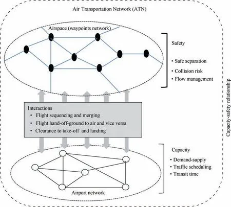
Fig. 1 Interactions and constraints of airport and airspace network in an ATN.

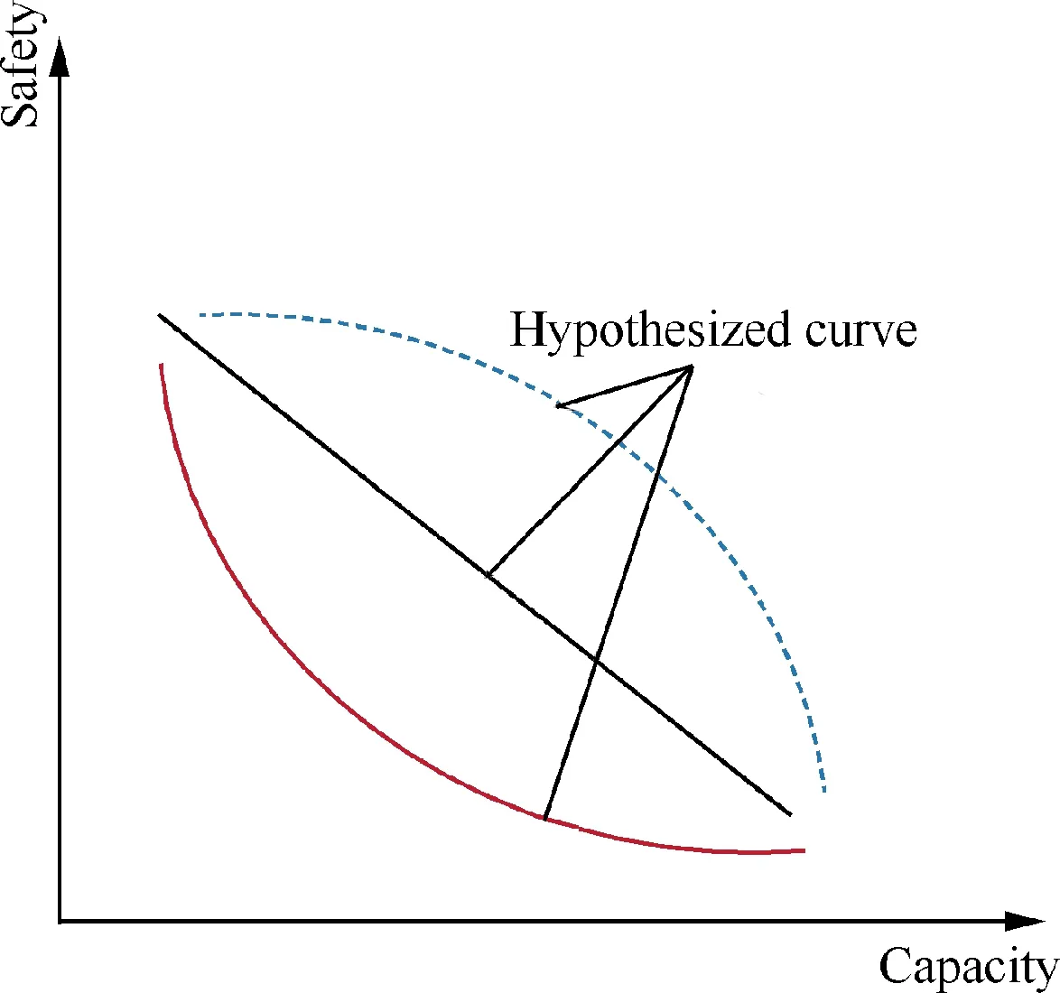
Fig. 2 Hypothetical safety-capacity relationship curves.

The airport network structure was abstracted to a directed,weighted network where nodes are the airports and edges are determined by flights.34Similarly, the airspace network is abstracted as a directed, weighted network where nodes are the waypoints and edges are determined by airways.35

3.1. Network generation

An ATN can be generated in two different ways(A)generate a network with two different type of nodes airports and waypoints and (B) generate the airport network and airspace network separately and then combine them together. Both of the approach will end up to a similar ATN, as a result we have considered the first approach only. To generate it we extend the technique developed by Mehadhebi36that consists of the following steps.

Firstly, a Delaunay triangulation network of Q points is created in a given area. In mathematics and computational geometry, a Delaunay triangulation for a set (Q) of points in a plane is a triangulation (DT (Q)) such that no point in Q is inside the circumference of any triangle in DT(Q).We apply the Delaunay triangulation algorithm37to create Q in a twodimensional plan with no overlapping connections among the points, each of which is an associated value of its latitude and longitude,to def ine its geographical location.Fig.4 shows a Delaunay triangulation network of Q=500 points in an area of 200 square nautical miles.

As, in a Delaunay triangulation network, some of the points tend to be very close to each other, we merge all the intersecting points that are too close. Although this will, in some way, increase the overall route distances, its benef it is reduced complexity of the ATN.

As we def ine an ATN as a combination of an airport network and airspace network (network of waypoints), the next step is to create the underlying airport network. Let V be a set of airports chosen randomly from Q (V ⊂Q) with the rest of the points (QV) def ine as waypoints. The connections among the airports (V) are developed using complex network generation models (random graphs38and small-world networks39) to create the topology of the airport network. In it,the connected airports are separated by at least 100 nautical miles so that a flight spends at least 70% of its travel time in the cruise phase. Fig. 5 presents an example of an airport network with 20 airports.

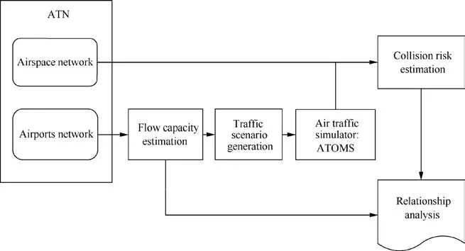
Fig. 3 Conceptual approach for analyzing capacity - collision risk relationship in an ATN.

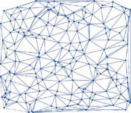
Fig. 4 Example of Delaunay triangulation network.

Finally, the ATN is constructed by combining the shortest paths among the directly connected airports along the Delaunay triangulation network. Letting P be the set of shortest paths for all the connected airports in the airport network,the ATN is defined as:

where piis the i th shortest path between any two connected airports in the network.

Fig. 5 Random airport network conf iguration generated from Delaunay triangulation point set (Q).

Fig.6 shows an ATN created from the Delaunay triangulation and airport network described in the above steps (filled squares(·)represents present airports and stearic(*)waypoints).

4. Methodology

Having generated the ATN,the methodology for analyzing the relation- ship between the airport network capacity and airspace network collision risk involves the following three key stages.

(1) Network capacity estimation The capacity of an ATN is defined as the maximum traffic that can be accommodated by its airport net-work subject to resource constraints, such as flow mix and node/link capacity,which determines the limit of feasible flow an air transportation network can accommodate. The flow intensity level is controlled by the wake-vortex separation minima,with an increase in the wake-vortex separation among aircraft during landing and take-off resulting in a decrease in the hourly flow in the ATN.

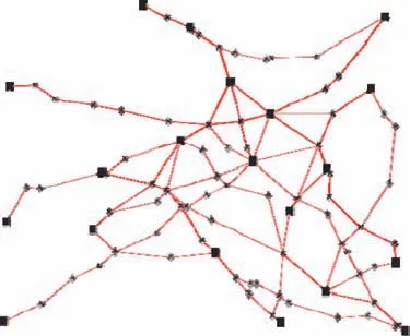
Fig. 6 ATN of 20 airports.

(2) Traff ic scenario generation with def ine flow intensity In this stage, given the flow, a complete traffic scenario is generated in a way that minimizes the overall collision risk using evolutionary optimization. In this paper we have used the term flow (flow intensity) and capacity interchangeably.(3) Collision risk estimation In any airspace, collision risk (the probability of two aircraft colliding per flight hour) is one of the key safety indicators as defined by the ICAO.10Collision risk is usually compared against a threshold value defined by ICAO,called Target Level of Safety (TLS), which provides a quantitative basis for judging the safety of operations in an airspace network.40The given traffic scenario is simulated in ATOMS to calculate the total number of flight hours and the probability of collision for each proximate pair of aircraft and, integrated with the Hsu model,41the overall collision risk is estimated.

Fig. 7 illustrates the process for analyzing the trade-off between the flow capacity and collision risk of a given ATN.It begins with a very large flow intensity and,once a traffic scenario is generated, the overall collision risk for that scenario is estimated.Then,the flow is increased and the process continues until the flow level reaches the maximum capacity bound.Once all the possible scenarios for different flow levels are evaluated, the repository data is subsequently analyzed to reveal the trade-off.

4.1. Network capacity estimation

Estimating capacity of an airport network system is a very hard combinatorial problem.A few numbers of attempts have been made to estimate the total capacity of an entire airport network system for any region or country.24,42Authors in Ref.26proposed a mathematical formulation and a heuristic solution for estimating the capacity of a given airport considering different flow mix and travel time. However, the model only consider a discrete travel time for all type of aircraft. In this paper we enhance the airport network capacity estimate model to accommodate different travel time for different aircraft as follows:

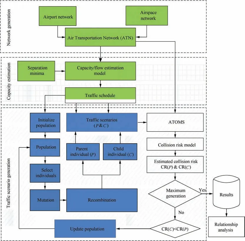
Fig. 7 Evolutionary framework for analysing capacity-collision risk relationship in ATN.

In this paper, we have used a time based separation minimum between landing-landing, taking off - taking off,landing-taking-off or vice-versa to avoid the wake-vortex turbulence which is given in the following Table 1.In addition to that we also introduce some extra separation(es)between two consecutive aircrafts. The value to extra separation (es) will serve as a control parameter to decease the maximum hourly flow in the network, when the value of es=0 the output of the capacity estimation module will provide the capacity upper bound (maximum attainable flow). The solution of an airport capacity will provide a list of flights and their schedule departure and arrival time that we called a traffic schedule.This traffic schedule then converted into a traffic scenario by assigning flight level, speed at different phase using a differential evolutionary optimization method and an air traffic simulator.

4.2. Traff ic scenario generation

Generating traffic scenarios using simple rules or hand scripting results very few alternatives from which it will be very hard to derive any conclusions.In this paper,we design a traffic scenarios generation method based on an airport network capacity estimation model26using an evolutionary framework.For a given traffic schedule,a complete traffic scenario must contain the tracks or air routes,feasible flight levels,and velocities and rates of climb and descent of different flight phases for all flights.Also,since the ATN is simultaneously shared by many aircrafts, the path of each and every aircraft needs to be conf lict-free.Therefore,converting the output from the airport networks capacity module (traffic schedule) to a traffic scenario is a complex task, to handle which we develop the following evolutionary computation framework.

4.2.1. Evolutionary computation framework design

Given an ATN and schedule of departures and arrivals of N flights and their routes,the problem of generating a traffic scenario involves determining the flight path levels of N flight that minimize the overall mid-air collision risk.Due to large search space (possibilities) and non-linear inter- actions between different components of air transportation system, maketraditional search methods, such as Monte Carlo, computationally infeasible.43Nature-Inspired techniques such as Differential Evolution (DE) algorithms have emerged as an important tool to effectively address complex problems in air transportation domain. Differential Evolution29is a stochastic, population-based optimization algorithm belonging to the class of Evolutionary Computation algorithms. Differential Evolution algorithms are highly effective in optimizing real valued parameter(traffic schedule in our case)and real valued function (minimize collision risk in our case). They are also highly effective in approximate solutions to global optimization problems (airspace collision risk in our case).

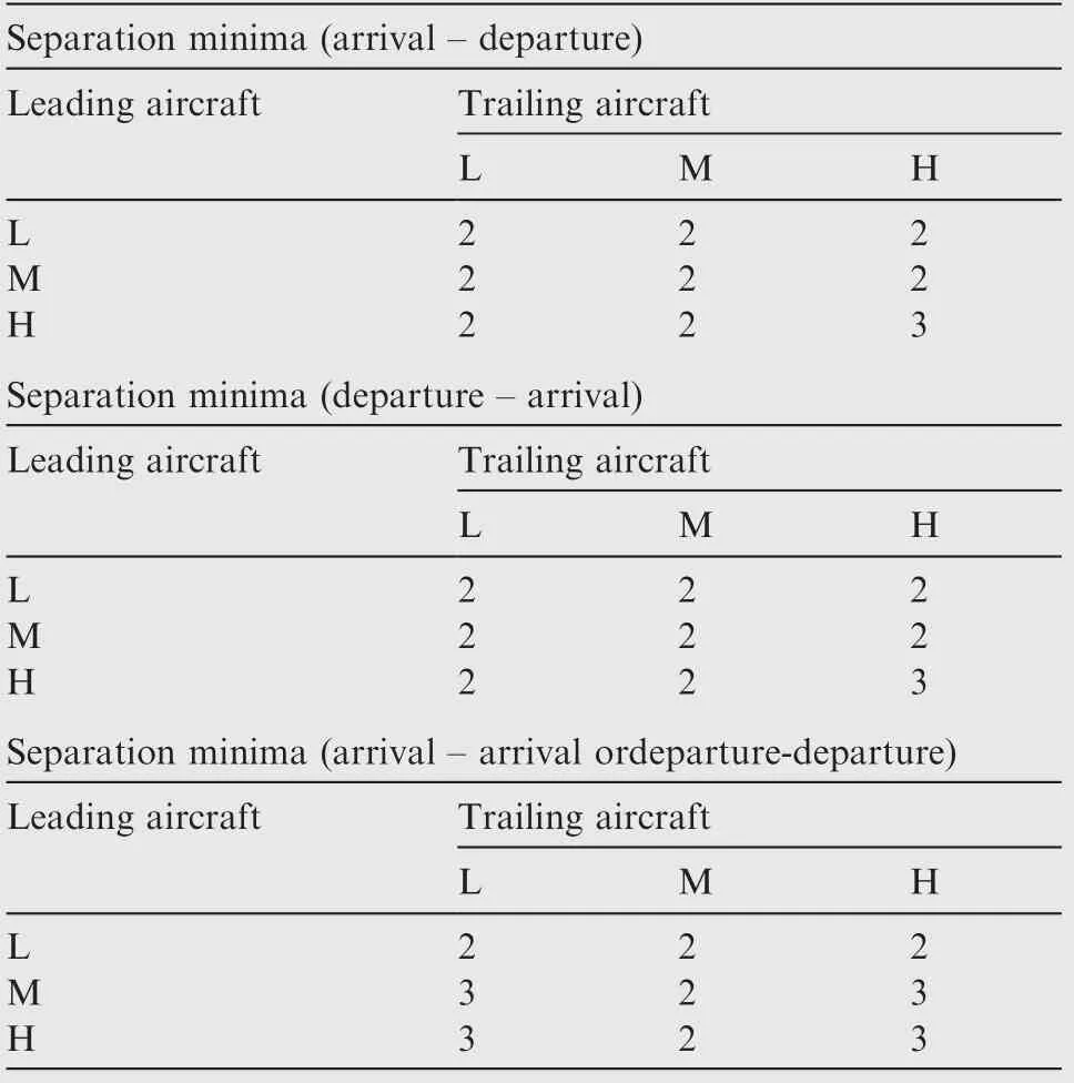
Table 1 Separation minima (in minutes) between aircrafts considered in this paper.

The proposed methodology for evolving flight level for each flight is illustrated in Fig. 7.To def ine the flight,we have used the shortest path from the origin to destination in the ATN for each flight.If there is more than one shortest path,one of them is chosen randomly and the flight levels evolved using a DE algorithm. In Fig. 7 green boxes depict the airport network’s capacity estimations which generate a traffic schedule, white boxes represent the air traffic simulation which evaluates a given traffic data for collision risk in an airspace and blue boxes represent the DE 2934process to evolve optimal flight levels.

The DE process begins by defined the upper and lower bounds of the flight path levels for each flight. It then undergoes a random initialization (within the bounds) of a population of solutions representing a set of vectors, where the size of each vector is equal to the number of aircraft defined by the traffic schedule.Each vector is considered a traffic scenario which is then simulated in ATOMS for its collision risk estimation,where the speeds of the flight in different stages are determined. After an initial evaluation, these vectors undergo mutation and recombination to generate two vectors we call the target and trial vectors which compete with each other.The one that minimizes the collision risk for the given traffic data is admitted to the next generation and the process continues until the maximum number of generations is reached.Then,the best-performing solutions(vectors)are selected from the final population.

(1) Representation of Flight Levels Since the objective of generating a traffic scenario is to evolve the right flight level for each and every flight for a given flight schedule, the flight level is encoded in a genetic inspired data structure (chromosome). Fig. 8 illustrates a set of chromosomes that constitutes the flight population in which each chromosome represents a set of flight levels to be applied to its corresponding flight; for example, if there are N flights, there will be N randomly assigned flight levels in a given chromosome. In this research, we do not consider semicircular rules of flying and we choose only flight levels FL290 (29000 ft) to FL-390 (39000 ft) which are encoded as real values from 2.9 to 3.9 with a precession of 1, from which the actual flight levels are calculated using the equation FL=(encoded value)×10000 ft.

(2) Fitness Function The role of a fitness function in an evolutionary algorithm (EA), Differential Evolution in our case, is to guide the search process by providing feedback on the quality of a solution represented by a chromosome in the population.Since this quality in our case depends on the estimated collision risk, we def ine the fitness as:

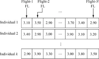
Fig. 8 Chromosome design with encoded Flight Level (FL) for each flight in given traffic scenario.

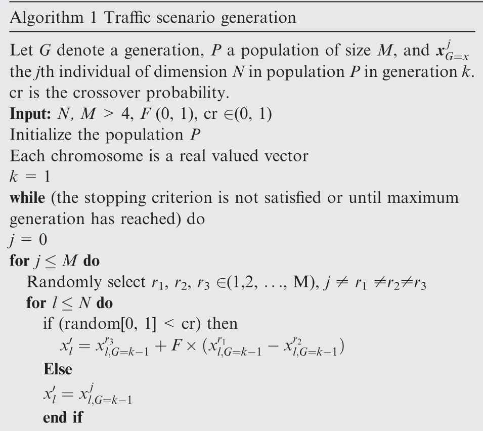
Algorithm 1 Traきc scenario generation Let G denote a generation, P a population of size M, and x j G=x the j th individual of dimension N in population P in generation k.cr is the crossover probability.Input: N, M ＞4, F (0, 1), cr ∈(0, 1)Initialize the population P Each chromosome is a real valued vector k=1 while (the stopping criterion is not satisfied or until maximum generation has reached) do j=0 for j ≤M do Randomly select r1, r2, r3 ∈(1,2, ..., M), j ≠r1 ≠r2≠r3 for l ≤N do if (random[0, 1]＜cr) then x′l =xr3 l,G=k-1+F×（xr1 l,G=k-1-xr2 l,G=k-1）Else x′l =x j l,G=k-1 end if

end for f（x′）=evaluate（x′）f（x jG=k-1）=evaluate（x jG=k-1）If f（x′）≤f（x jG=k-1） then x j G=k-1 =x′Else x j G=k =x jG=k-1 end if end for k=k+1 end while

5. Experimental setup

In the experiments, we control the flow in the network by changing the extra separation parameter (es), starting with a low flow of es=20 and then gradually decreasing it by 1.For each es value, we generate 20 different traffic scenarios,each with the following parameter settings, using the evolutionary framework with different seeds and then estimate the collision risk.

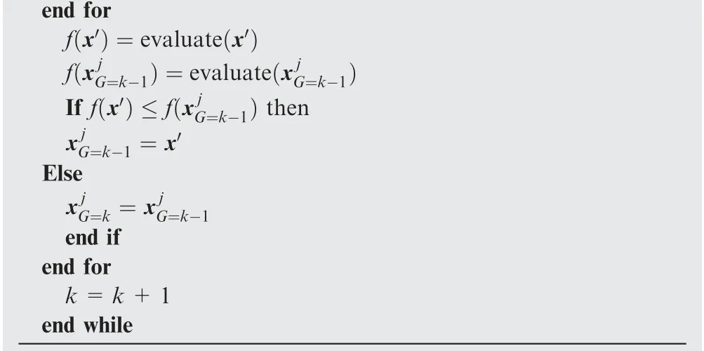
(1) Test Network In order to assess the effectiveness of the proposed airport network capacity estimation model, we perform experiments on two different types of test network: (i)ATN-I in which the airports and their connectivity are chosen randomly; and (ii) ATN-II in which the locations of the airports are placed on the circumference of a circle and their connectivity created using the small-world model [39]. Both these networks consist of 20 airports, as shown in Fig. 9, with the difference between them their airport network topologies as ATN-I is considered a random and ATN-II a smallworld network.

(2) Collision Risk Parameters The Collision Risk models parameters are set as follows:Vertical overlap probability Pz(0)=0.55,vertical speed when in horizontal flight|z˙|=1.5 m/s and aircraft position update time Tmin=0.16 min. The diameter of aircraft cylinder (aircraft safety protection volume) is set based on the aircraft type of the proximity pair as shown in Table 2, whereas, the height of the cylinder is set toλz=55 m for all cases.

(3) Evolution Parameters In our experiments, we use a population of 50 individuals and DE mutation factor (F) of 0.40. We conduct a series of experiments to determine the maximum number of generations for stopping and the proper crossover rate by running the evolution for up to 500 generations using different crossover rates.Fig.10 shows the best f it values(minimum collision risks)of the population over generations from which it is clear that, after 350 generations,the best individual value does not improve in all cases.Therefore,as we can say that 400 generations is suff icient to converge the evolution process, this is set as the stopping criterion for the DE process in the subsequent analysis.

Fig. 9 Layout of test ATNs.

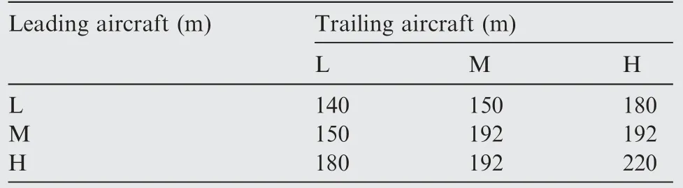
Table 2 Diameters of cylinder for different proximity pairs.

Fig. 10 Selection of evolution parameter (maximum generation and crossover rate).

In order to determine a proper crossover rate, we perform experiments with different ones. Fig. 11 shows the best fitness values after the final generation for different crossover rates(cr) ranging from 0.40 to 0.95 with an increment of 0.05 after 500 generations which indicates that the best f i value is the lowest for a crossover rate of 0.80.Therefore,we set the crossover rate for DE to 0.80 for the subsequent analysis.

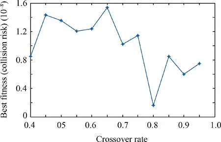
Fig. 11 Best fitness values after final generation with different crossover rates (cr).

6. Results and analysis

We first present the characterization of the test ATNs. In the test ATN-I, the underlying airport network has a uniform degree distribution, which is shown in Table 3. In the ATNII,the small-world topology of airport network is created with a staring ring lattice where every node is connected to its K=4 neighbors (K/2 on either side), where K represent the mean degree of the network, then it under goes a random rewiring with a probability of 0.05.Apart from the connectivity pattern we also present the distance in nautical miles among the connected airports and number of way-points along the shortest path between them for ATN-I and ATN-II in Tables 4 and 5 respectively. From Tables 4 and 5 it is clear that the minimum distance among the airport’s links are 100.51NM and 101.59NM for ATN-I and II respectively.

In each ATN,the traffic schedule consists oflight;medium and heavy aircraft generated using the capacity estimation module and then converted into a traffic scenario by the evolutionary optimization method.Fig.12 presents the maximum attainable flows in the test ATNs over a period of 24 h.

As,for a given flow,there will be many solutions because of the combination oflight, medium and heavy aircraft, we generate 20 traffic scenarios in every case. In our experiments, we control the flow by the extra separation parameter(es).Tables 6 and 7 summarize the average hourly traffic densities (hourly flight movements) for test networks ATN-I and ATN-II respectively. Their maximum hourly traffic flows (capacity)are found to be identical while the small-world conf iguration(ATN-II) can accommodate higher traffic than its random counterpart (ATN-I).

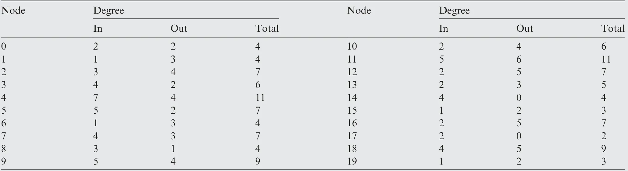
Table 3 Connectivity of the airports in ATN-I.

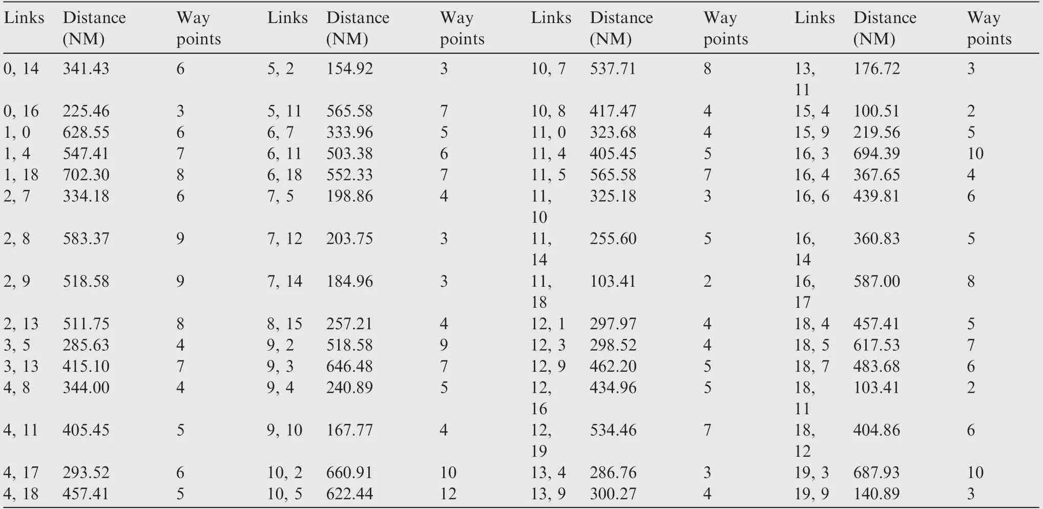
Table 4 ATN-I link’s distance and number of way points.

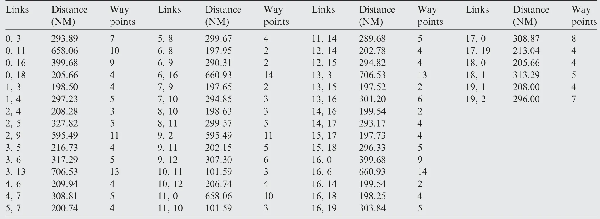
Table 5 ATN-II link’s distance and number of way points.

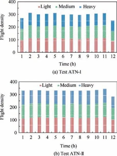
Fig. 12 Hourly flow of test ATNs for es=0.

For a given flow the output from the capacity estimation module is converted to a traffic scenario by a DE process,with the purpose of assigning flight levels for each that minimize the overall collision risk,while the speed and other parameters are set by ATOMS.Fig.13 shows the percentages of usage of each flight level averaged over 20 scenarios determined by calculating the total number of flight flows through a scenario divided by the total number of flights in it.It is clear that all the flight levels are almost equally utilized except for some traffic scenarios with es=18 in which flight levels FL 290 and FL390 are the most used in ATN-I and ATN-II respectively.

Fig.14 shows the collision risk of each test ATN as a function of the hourly flows.As the number of hourly flight movements increases, all collision risks increase almost linearly for both cases, with the average collision risk always more for ATN-I than ATN-II. In both cases, the collision risk hits the TLS (1.5×10-8)44as the hourly flight movements among the airports increase which we call the critical flow,with those of ATN-I and ATN-II 135 and 115 (hourly flight movements)respectively.

7. Conclusions

With the aim of increasing the capacity and enhancing the safety of air transportation, this paper proposed a framework for airport and airspace network interaction with the aim of analyzing the trade-off between capacity and safety. The proposed methodology was tested on two different ATN topologies random (ATN-I) and small-world (ATN-II) with the same number of airports.

The experimental results indicated that,if the airspace TLS was relaxed,the maximum hourly flow(capacity)of the smallworld conf iguration (ATN-II) could accommodate more traf-f ic than the random one (ATN-I). In both cases, as the flow increased in the airport network, the overall airspace’s collision risk increased linearly and crossed the TLS because,although the airport network system could handle more traffic,the safety barrier of the airspace served as a bottleneck in terms of the overall capacity of the air traffic network. Therefore, estimating the true capacity of an air transportation network system without considering safety is very unrealistic as its maximum capacity depends on the interactions of its underlying airport network and airspace waypoints network.

Table 6 Hourly flight movements in the test ATN I.

Table 7 Hourly flight movements in the test ATN II.

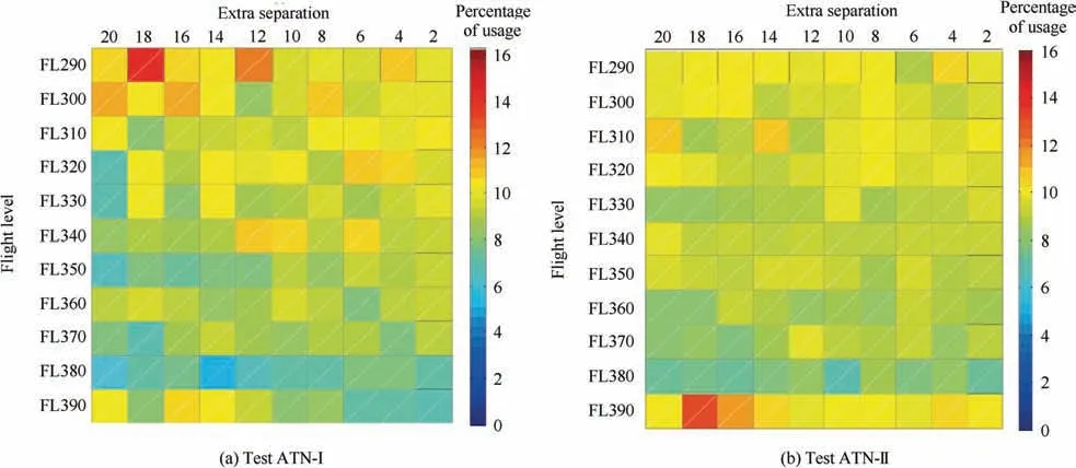
Fig. 13 Percentages of usage of different flight level.

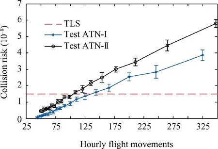
Fig. 14 Capacity-collision risk relationship.

It was found that, in general, the capacity upper bound depends not only on the connectivity among airports and their individual performances but also the conf iguration of waypoints and mid-air interactions among flights. We demonstrated that, as the hourly flow in the network increased after a certain level,the overall collision risk crossed the TLS which we def ine as the critical flow for the given ATN. However, as the location of the critical point depends on the particular network conf iguration,it may vary from network to network.The critical flow of the random topology(ATN-I)was found to be larger than its small-world counterpart while, in terms of airspace safety,its collision risk was smaller for the same flight.These results may facilitate decision-makers in gaining insights into how capacity and safety interact with each other,discovering system bottlenecks and using such knowledge to improve an ATN’s performance and sustainability.