A Graph-Based Reinforcement Learning Method with Converged State Exploration and Exploitation

Han Li,Tianding Chen ,Hualiang Teng and Yingtao Jiang

Abstract: In any classical value-based reinforcement learning method,an agent,despite of its continuous interactions with the environment,is yet unable to quickly generate a complete and independent description of the entire environment,leaving the learning method to struggle with a difficult dilemma of choosing between the two tasks,namely exploration and exploitation.This problem becomes more pronounced when the agent has to deal with a dynamic environment,of which the configuration and/or parameters are constantly changing.In this paper,this problem is approached by first mapping a reinforcement learning scheme to a directed graph,and the set that contains all the states already explored shall continue to be exploited in the context of such a graph.We have proved that the two tasks of exploration and exploitation eventually converge in the decision-making process,and thus,there is no need to face the exploration vs.exploitation tradeoff as all the existing reinforcement learning methods do.Rather this observation indicates that a reinforcement learning scheme is essentially the same as searching for the shortest path in a dynamic environment,which is readily tackled by a modified Floyd-Warshall algorithm as proposed in the paper.The experimental results have confirmed that the proposed graph-based reinforcement learning algorithm has significantly higher performance than both standard Q-learning algorithm and improved Q-learning algorithm in solving mazes,rendering it an algorithm of choice in applications involving dynamic environments.

Keywords:Reinforcement learning,graph,exploration and exploitation,maze.

1 Introduction

Reinforcement Learning (RL) has found its great use in a lot of practical applications,ranging from problems in mobile robot [Mataric (1997);Smart and Kaelbling (2002);Huang,Cao and Guo (2005)],adaptive control [Sutton,Barto and Williams (1992);Lewis,Varbie and Vamvoudakis (2012);Lewis and Varbie (2009)],AI-backed chess playing [Silver,Hubert,Schrittwieser et al.(2017);Silver,Schrittwieser,Simonyan et al.(2017);Silver,Huang,Maddison et al.(2016)],among many others.The idea behind reinforcement learning,as illustrated in Fig.1,is that an agent learns from the environment by interacting with it and receives positive or negative rewards for performing calculated actions,and the cycle is repeated.The key issue of the whole process is to learn a way of controlling the system so as to maximize the total award.

When the agent begins to sense and learn a completely or partially unknown environment,it involves in two distinct tasks:exploration which attempts to collect as much information about the environment as possible,and exploitation which attempts to receive positive rewards as quickly as possible.

There is a dilemma of choosing between the two tasks of exploration and exploitation,though.Too much exploration will adversely influence the efficiency and convergence of the learning algorithm,while putting too much emphasis on exploitation will increase the possibility of falling into a locally optimal solution.The existing RL algorithms all attempt to balance out these two tasks in their learning cycles (Fig.1),but these is no guarantee that the best result can always be obtained.

Besides the exploration and exploitation dilemma,the RL algorithms have to employ value distributions that inexplicitly assume that environment is static (i.e.,no change),or it changes very slowly and/or insignificantly.However,in many real applications,the environment rarely stays unchanged.More than likely,the environment that can be described in terms of states (Fig.1) changes over the course of exploration.In this case,value distribution has nothing to do with the problem at hand,and all the information obtained from the previous exploration efforts become less,or totally irrelevant.

To effectively solve the aforementioned problems in reinforcement learning,we herein present a new algorithm based on the partitioning of the states set and search of the shortest path in a directed graph that represents a RL method.We have formally proved and experimentally verified that both exploration and exploitation in reinforcement learning actually converge at the end of the decision-making process,and thus,the learning process does not need to face the exploration/exploration dilemma as other existing reinforcement learning methods would do.This observation indicates that a reinforcement learning scheme is essentially the same as searching for the shortest path in a dynamic environment,which is readily tackled by a modified Floyd-Warshall algorithm as proposed in the paper.The experiment that applies the proposed algorithm to solve mazes confirm better performance of the new algorithm,particularly its effectiveness in addressing issues pertaining to a dynamic environment.

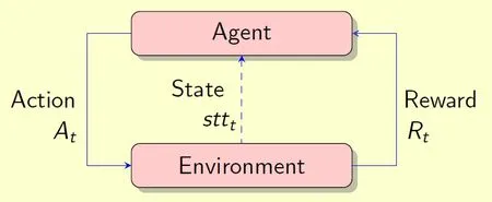
Figure 1:In reinforcement learning,the agent observes the environment,takes an action to interact with the environment,updates its own state and receives reward

2 Preliminaries and background

In this section,we will first survey the basic structure of reinforcement learning (RL) algorithms,particularly value-oriented method of RL,and formally define the explorationvs.exploitation tradeoff in RL.In the literature,RL is shown to be mapped to various graph representations,and these methods are briefly described in the section as well.With graph representations,RL can benefit from rich results in graph algorithms,and we thereby finish this section by reviewing algorithms that search for the shortest path in a graph,as they are related to this paper.

2.1 Value-oriented method for the exploration-exploitation tradeoff in RL

Most RL problems can be formalized using Markov Decision Processes (MDPs),and there are a few key elements in RL as defined below.

1.Agent:An agent takes actions.

2.Environment:The physical world through which the agent operates.

3.State:A state is a concrete and immediate situation in which the agent finds itself.In this paper,we denotesttias the state of the agent at time instancei,and setScontains all the states that the agent can operate on.That is,stti∈S.

4.Action:agents choose among a list of possible actions.Denote aias the action that agent might perform at time instance i.Actions is defined as the set of all possible moves of the agent can make,i.e.,ai∈Actions.

5.Reward:A reward is the feedback that is used to measure the success or failure of an agent’s action.Here a reward at time instance t is defined as Rt.Actions may affect both the immediate reward and,through the next situation,all the subsequent rewards [Sutton and Barto (2017)]

6.Exploitation:a task that makes the best decision given all the current information.

7.Exploration:a task that gathers more information to be used for making the best decision in the future.

8.An episode:the behavior process cycle of the agent from the beginning of the exploration to the beginning of the next exploration.When the interaction between the agent and the environment breaks naturally into subsequences,which are referred as episodes.Each episode ends in a special state called the terminal state,followed by a reset to a standard starting state or to a sample from a standard distribution of starting states [Sutton and Barto (2017)].

In RL,the exploration-exploitation tradeoff refers to a decision making process that chooses between exploration and exploitation.Value-oriented RL methods have to deal with such exploration-exploitation tradeoff through the value distribution as defined by the value function or a probability that decides the chain of actions that lead to the target state all the way from the start state through a series of awards.A decision chain refers to a series of decision-making steps taken by an agent.

In order to strike a balance between exploration and exploitation,there are two main decision methods that can be followed,the ϵ-greedy and softmax.

In ϵ-greedy method,the action is selected by,one has

where astt∗is the action in which of the value function assumes the highest value:

where Q(stt,a) is action-value function which evaluates each possible action while in the current state.One drawback of ϵ-greedy action selection is that when it explores,all the possible actions are given the equal opportunity,as indicated in Eq.(1).In a simple term,this method is as likely to choose the worst-appearing action as it is to choose the next-to-best action.This gives rise to the so-called softmax method that can vary the action probabilities through a graded function below,

where π(a|stt) is the probability policy to choose an action from the specific state stt,and τ is a “computational” temperature,and is an action-value function that evaluates each possible action in the current state.

The problem of value-oriented method is due to its weak ability to eliminate exploration blindness resulting from a large number of repeated explored states introduced by the value distribution structure.The stochastic factors that are added to help the search process jump out of the loops and balance exploration and exploitation actually come at the expense of more blindness of exploration.

2.2 RL over graphs

A RL can be represented as a directed graph,G,where a vertex,vi∈V(G),corresponds to a state sttiin reinforcement learning and an edge,eij∈E(G),connects two vertices (two states sttiand sttj) with a decision action aiin reinforcement learning.In this graph,a path can be regarded as decision sequences in reinforcement learning.

In the literature,many RL methods are related to their graph representations.In PartiGame Algorithm [Moore (1994)],the environment of RL is divided into cells modeled by kd-tree,and in each cell,the actions available consist of aiming at the neighbor cells [Kaelbling,Littman,Moore (1996)].In Dayan et al.[Dayan and Hinton (1993)],speedup of reinforcement learning is achieved by creating a Q-learning managerial hierarchy in which high-level managers learn how to set tasks for their lower level managers.The hierarchical Q-learning algorithm in Dietterich [Dietterich (1998)] proves its convergence and shows experimentally that it can learn much faster than ordinary "flat" Q-learning.None of these methods,however,can solve the root problem concerning the dilemma of exploration and exploitation.

2.3 Floyd-Warshall algorithm

Denote SSA(G,ei,ej) as a shortest path search algorithm that is applied toG from verticeeito verticeejthat represents a RL.The classical shortest path algorithms like Dijkstra[Dijkstra (1959)] and A* [Hart,Nilsson,Raphael (1968)] are single starting point algorithms for the path-finding.The Floyd-Warshall algorithm [Floyd (1962)] (FW),which is pursued to use in this study,provides the shortest path between any two vertices in specified graph and it is found to be adaptive to the change of the graph.

In the standard Floyd-Warshall algorithm,two matrices (DIST and NEXT) are used to express the information of all the shortest path in the graph.The matrix DIST records the shortest path length between two vertices.The matrix NEXT contains a name of the intermediate vertex through which the two vertices are connected through the shortest path.Because of the optimal substructure property of the shortest path,no matter how many intermediate vertices the shortest path passes through,simply recording one of the intermediate vertices is sufficient to express the entire shortest path.

3 Convergence of exploration and exploitation

In this section,we first define the completely explored graph,which serves as the foundation for a graph-based iterative framework for reinforcement learning.Under this framework,the acquired knowledge from the RL’s exploration task can be recorded by the graph,and the shortest path search can then be conducted to determine the next decision chain.This new approach is able to well track the graph changes that are caused by exploration and sometimes by the changing environment.In this section,we shall prove that with this framework involving the shortest path search,the exploration actually converges to exploitation.In a simple word,exploration will find the shortest path to reach the same reward as exploitation does.

3.1 Completely explored graph

Definition 1 ACompletely Explored Stateis a state of which all its possible successor states have already been explored.If one of a state’s successor states has been explored and at least one of its successor states has not yet been explored,the state is called aPartially Explored State.

Definition 2 If the vertex set V in connected graph Gincludes the start states of episodes and all these states have been completely explored,and the edge set E represents all the actions that need to be taken to connect all the different states,graph G is called aCompletely Explored Graph(CEG).

Fig.2 shows an example of a CEG where each state (sttxx) is linked with up to 4 possible actions:a0,a1,a2,a3.There are some explored edges which are omitted for simplicity,such as action a1for (stt20) and (stt01)witℎ a0;they point to nonexistent state transitions.

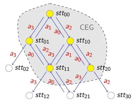
Figure 2:An example of a completely explored graph.Nodes represent states and directed edges between nodes represent actions.The shadowed area that includes all the State nodes (colored yellow) and all the associated directed edges represents the CEG.The unfilled nodes outside the shadowed area represent incompletely explored states,even though they connect to the CEG

Suppose the complete actions set Actions={ai:a0,…,an} is known.State sttiis a completely explored state if any reachable next state of stti,denoted as stti+1,by taking a possible action ai∈Actions,is traversed.LetGUrepresent a graph that contains all the traversed states,including both the completely and the partially explored states.We can definethe predecessor state setSetpredecessor(stt)as

Setpredecessor(stt)={s:(s ∈SE)∧({s,stt}∈E(GU))} and the successor state set

Setsuccessor(stt) is defined as

Setsuccessor(stt)={s:s ∈SE ∧{stt,s}∈E(GU)} where SE denotes the set V(CEG).

If we denote an environment feedback function byEnv,then for a given actionak,the next statesi+1can be determined assi+1=Env(si,ak).

3.2 Exploration converges to exploitation

From CEG,we can prove that exploration converges to exploitation.Here sttrwdis denoted as a reward state.

Lemma 1.Suppose that exploration of each episode starts with state stt0,and ends in reward state sttrwdafter passing some intermediate states through a series of episodes.Of all the possible episodes,one can see sttrwd∉SE.

Proof:Once the agent has landed in state sttrwd,the episode ends,so there will be no further exploration originated from sttrwd.That is,the graph is a completely explored graph and the states are completely explored states,according to definitions 1 and 2.Thus sttrwdcannot be a member of the SE set.(End of proof)

Define the envelope set of set SE asSEE ={stti:(sttiSE)∧(Setsuccessor(stti)⊄SE)}Corollary 1.For stti∈SEE consists of members in SE,there exists at least one of the successor states of sttidoes not belong to SE.

Proof:It comes directly from the definition of SEE.(End of proof)

Corollary 2.If stti∈(Setpredecessor(sttrwd)∩SE) is in an exploring episode,then irrespective of the explore strategies adopted in the future,sttiwill always be part of SEE.Proof:From lemma 1,one can see that if stti∈SE has a successor state sttrwdand it is impossible for sttrwdto be a member ofSE.By definition of SEE it is known that sttiis always a member of SEE.(End of proof)

Definition 3.If SSA(CEG) plans a decision chain that eventually reaches sttrwd,and it does not produce any change in either V(CEG) or E(CEG),this condition is referred asExploration Convergence.

Corollary 3.Once the exploration converges,the planned decision chain from SSA(CEG) remains the same in the next exploration episode.

Proof:At the beginning of each episode,a CEG is constructed as needed to explore the new states.If the CEG keeps unchanged at the end of the current episode,the next episode will produce the exactly same path.At this point,the algorithm converges as it satisfies the condition set by Definition 3.(End of proof)

Theorem 1.Assume there are a finite number of states and a SSA(CEG) is able to find the shortest path in CEG,exploration becomes finding a path from the start state stt0to the sttrwd.In other words,exploration converges to exploitation.Proof:

i.During exploration,state stt0can reach the SEE through SSA(CEG) .That is,one needs to find the shortest path,pathk,among all the paths,such that:

where L(stti,sttj) is the length of the shortest path between state sttiand state sttj.

If sttk∈Setpredecessor(sttrwd),then (stt0,…,sttk,…,sttrwd) from SSA(CEG)algorithm marks the shortest path from stt0to sttrwd.In this case,the conditions concerning exploration convergence (defined in Definition 3) are met,and the exploration converges to the exploitation.

ii.If sttk∉Setpredecessor(sttrwd) ,CEG continues to evolve as exploration progresses.

iii.As exploration continues,new members are added intoSEEand they replace the old ones,extending the shortest path,and according to Corollary 2,any new member stti∈(Setpredecessor(sttrwd)∩SE) will always be part ofSEE.

iv.When exploration ends,sttkthat satisfies Eq.(4) will eventually meet the condition:sttk∈Setpredecessor(sttrwd) .

v.The agent is bounded to pass the state sttkassociated with the shortest path in the Setpredecessor(sttrwd.If not,there would have a different sttks∈Setpredecessor(sttrwd) from sttkthat otherwise makes L(stt0,sttks)＜L(stt0,sttk).If sttks∈SEE,it’s impossible forSSA(CEG)to choose sttkas a state in the shortest path.If sttks∉SEE,there must be a state sttm∈SEE in sttks’s predecessor chain that makes L(stt0,sttm)＜L(stt0,sttk).The algorithm does not converge during this episode.

vi.Putting all things together,one can see that exploration bySSA(CEG)must converge to the shortest path from start state stt0to sttrwd.

As indicated in corollary 3,once the algorithm has found the shortest path from stt0to sttrwd,the path will be repeated with no change in the following episodes.In this case,the exploration is readily to be halted.(End of proof).

4 Algorithm implementation

Based on Theorem 1 described in the previous section,we propose a framework for RL that does not need to concern about the dilemma of exploration and exploitation.There are two major components in the framework,namelyCEGand Incompletely explored states,and there are two iterative steps as illustrated in Fig.3:

i.Based on the currentCEG,an action decision,in the form of a single decision or a chain of multiple decisions,will be made to guide the next exploration.

ii.Update theCEGwith the new knowledge acquired from the latest exploration.In a static or nearly static environment,exploration will help continue to growCEG,while in a changing environment,CEGmembers can be added or deleted according to the exploration result.Note that when the CEG is updated,nodes or edges can be added or deleted from the graph.In a static environment,as the exploration progresses,the number of nodes and edges tends to increase,while in a dynamic environment,the number of nodes and edges may increase or decrease.

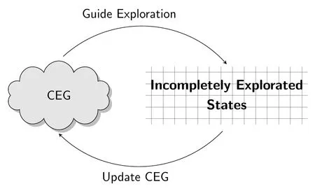
Figure 3:Graph iterative frame

4.1 Shortest path search in dynamic environment

The standard Floyd-Warshall Algorithm calculates matrices DIST and NEXT in batch divided by the length of short path (the number of relay vertices here) for each vertex pair.For constantly changing of vertices and graph structure that engages in exploration all the time,a more efficient method is needed and thus proposed in this section.

During exploration in reinforcement learning,the completely explored states are discovered in sequence,and subsequently,they are added to the CEG,after which the corresponding edges are also added.In addition,if the agent wants to adapt to the dynamic environment,the removal of vertex must also be taken into account.In this section,a modified algorithm Floyd-Warshall algorithm (SFW) is presented,which is able to search for the shortest path in a graph that represents a dynamic environment.In a simple term,we present SSA(CEG) for SFW.

In SFW,each time when a new vertex is added,it is not only to add the shortest path associated with the new vertex directly tied to the two matrices as defined in Floyd-Warshall,but also to compare the length of the new path introduced by the new vertex against that of the shortest path obtained from the prior iteration.These operations may result in the update of the two matrices.The major steps of SFW are summarized follow.If current statesttis to be added to setSE,do the following steps:

i.Add and initialize a new row in matrices DIST and NEXT.

ii.Add and initialize a new column in matrices DIST and NEXT.

iii.Update the new column by computing the shortest paths from all the vertices to this new vertex.

iv.Update the new row by computing the shortest paths from the new vertex to all the other vertices.

v.Update matrices DIST and NEXT by comparing the length of each vertices pair between the old shortest path recorded in the matrices and that of the new paths with the new vertex added.

Denote Lset(stti,Setpredecessor(stt)) as the length of the shortest path from arbitrary state sttito Setpredecessor(stt) as defined in Section 2:

Matrices DIST and NEXT are updated by performing the following operations:

where jminis the the result ofsttj∈Setpredecessor(stt)} as given in Eq.(5).

In the same token,one can update the stt’s predecessor states set Setpredecessor(stt)with stt’s successor states set Setsuccessor(stt).That is,

Correspondingly,matrix DIST in this case can be updated by

If a path that passes through state stt is shorter than the previously obtained shortest path,then matrix NEXT is updated by:

4.2 Guided exploration

As proved in Section 3,exploration finally converges to the shortest path that connects with the target state.Since exploration and exploitation basically produce the same result,our algorithm only needs to consider one single task,exploration.

The steps of how to guide exploration is listed in Tab.1.

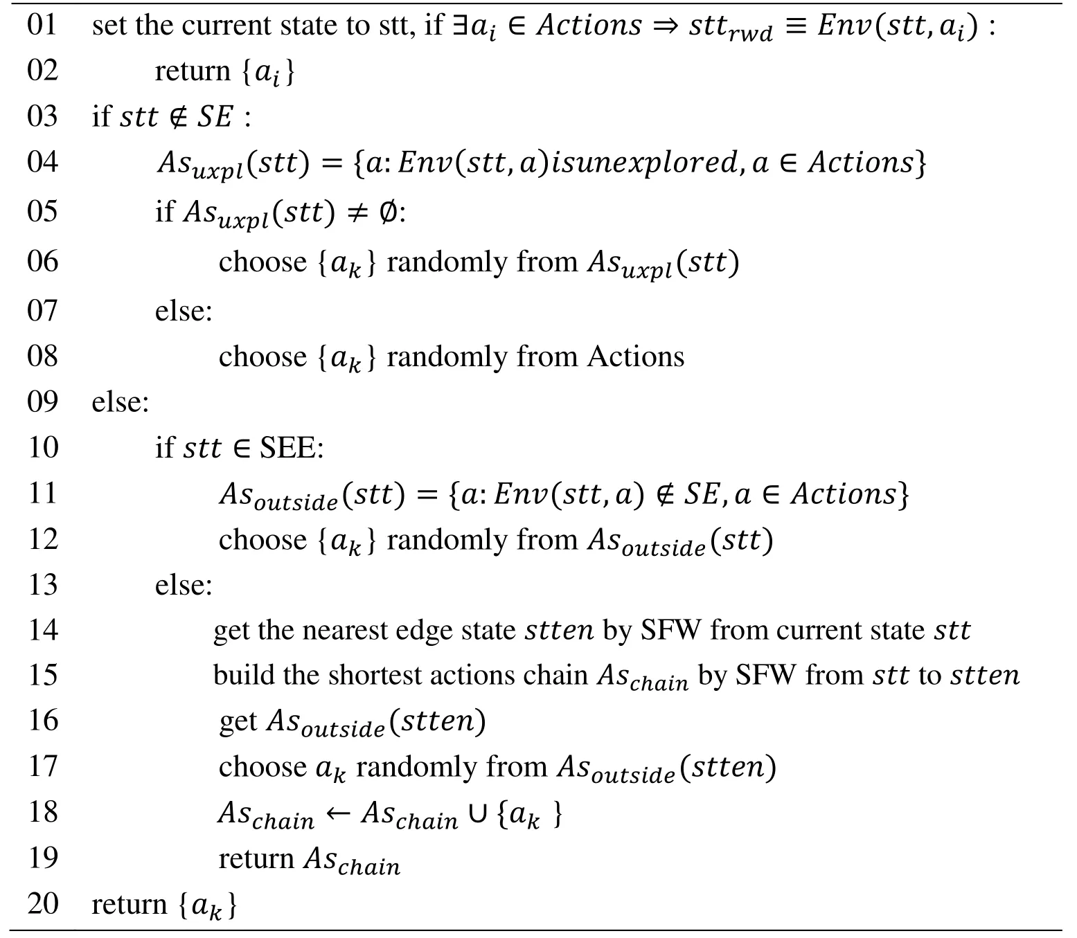
Table 1:Exploration algorithm

There are several major steps in the algorithm listed in Tab.1:

Step 1:If stt is a neighbor of sttrwd,the agent can take action aidirectly,which transitions the state to sttrwd.

Step 2:If stt is not a member ofSE,a decision is randomly made by calling Asuxpl(stt).

Step 3:If stt is an edge state ofSE,a decision is randomly made by calling Asoutside(stt).

Step 4:If stt is a member of SE but not a member of SEE,the shortest path is obtained using SFW.This path represents the decision chain by which the agent can exit SE in the most efficient way.

4.3 Update of the CEG

Before exploration starts,SEis empty,the agent has noa prioriknowledge of the environment.Denote stt0as the start state of each exploration episode.Once exploration begins,from the initial state stt0,for each successor state stti,an action akis selected from the actions set according to SFW,after which the agent moves to the next state stti+1by taking action akobtained from the feedback of the environment.

Exploration gets repeated.Whenever a new state is found,it will be added to the graph,GU,immediately.When the current state is completely explored,it will be added to setSE,sometimes to theSEEsimultaneously.This algorithm is listed in Tab.2.One can see that when a new completely explored state,corresponding to a vertex in the graph can be added to the CEG,it must generate some action decision reflected as edge changes in the graph.The new SEE by definition can be readily derived from the updated CEG.

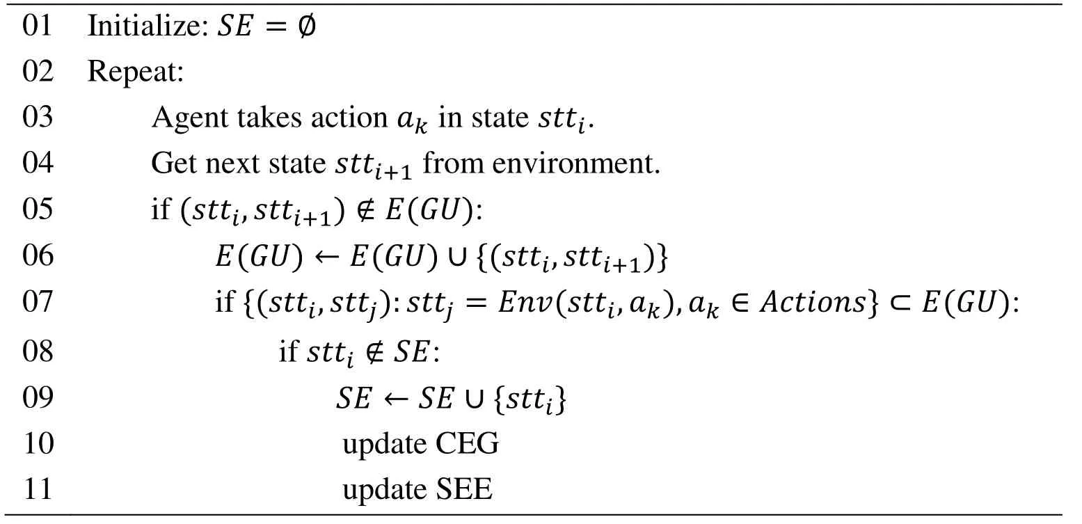
Table 2:Algorithm:update CEG

4.4 Notes on the proposed algorithm

If the current state of the agent is inSE,the shortest path to the boundary of the explored region is selected,as seen from the algorithm listed in Tab.1.As far as the completely explored states are concerned,our approach is able to traverse all of them as opposed to explore them repeatedly.In the classical Q-learning algorithm,there are such a large number of states that have to be traversed repeatedly.This subtle difference makes our algorithm more computationally efficient,as evidenced by the experimental results reported in the next section.

Compared to value-oriented algorithms,experiences in our approach obtained from exploration history are recorded inGUandSErather than derived from the value distribution.The establishment of two matrices in SFW relies onGUandSE,while its structure contains the shortest path of all the pairs of states in SE.Therefore,in the case of changing environment,the modest modification ofGUandSEand the updates of the two matrices will make the proposed algorithm more adaptive to the new,changing environment.This feature can be clearly seen from the result reported in 0.

5 Experimental results

The new graph-based algorithm detailed in Section 4 has been applied to solve a maze.Maze solving has been widely adopted for the testing of reinforcement learning algorithms.The agent in the experiment can be seen as a ground robot roaming in a maze,and it can always sense its current position (state) as it moves around.At the beginning of experiment,the agent knows nothing about the maze,and it needs to find the reward(target) position and complete its journey by passing through a path from a specified start position.

5.1 Setup of experiment

The maze has a size of 16 rows by 16 columns for a total of 256 blocks.There are 4 types of blocks,namely target,trap,obstacle and ordinary pass.The fixed start position is treated as a normal pass block.The agent gets a reward of 1 when it reaches the target,but if the agent falls into a trap,it will get a reward of -1.Both conditions will lead to the finish of current episode,and the agent will have to return to the start position and restart its exploration.Note that the agent can keep the exploration information from all the previous episodes.There are 975 mazes in the experiment,and they differ from each other in terms of the locations of the obstacle blocks.In our experiment,there are 46 obstacles for each of the 975 mazes.

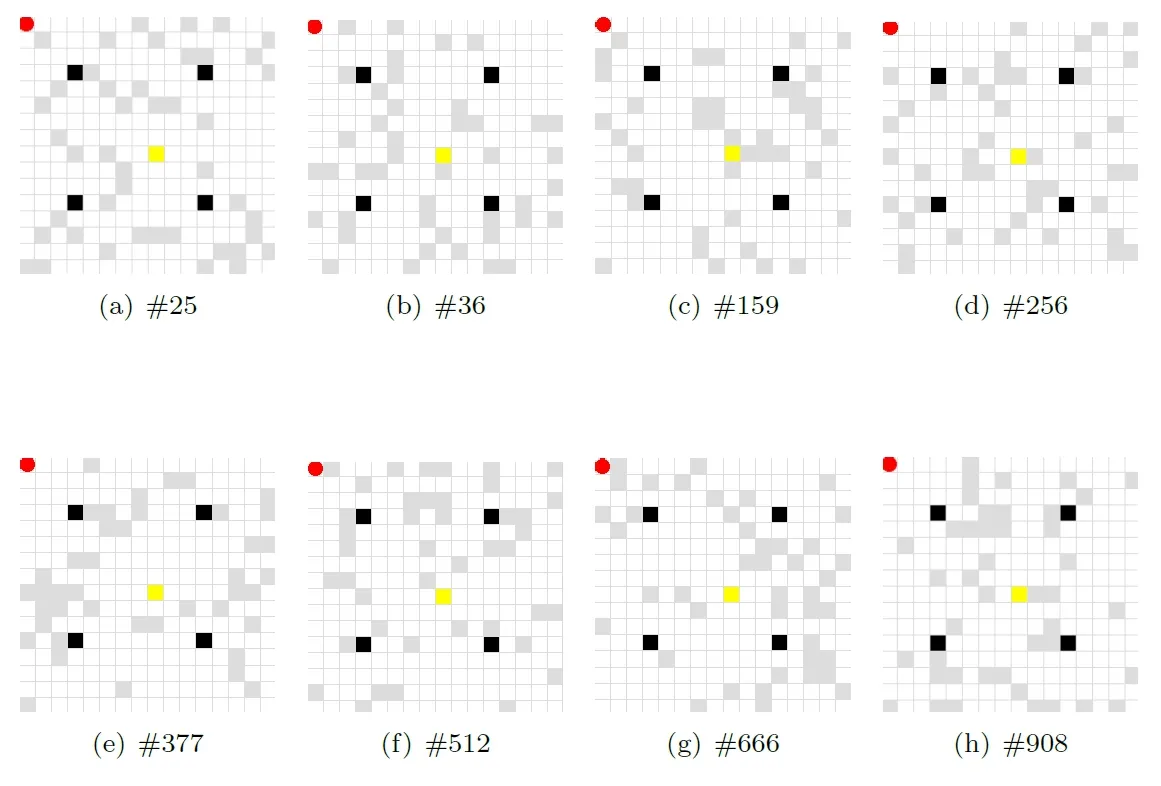
Figure 4:Maze settings

For each maze,the initial position of the agent is at the upper left corner (1,1),and the target position is set to be (9,9).There are 4 fixed traps,located at (4,4),(12,4),(4,12) and (12,12).Tab.3 summarizes the main characteristics of the maze.Fig.4 illustrates a sample of mazes,and their respective reference numbers are 25,36,159,256,377,512,666 and 908.In these mazes,the red circle represents the agent,gray blocks represent obstacles,black blocks represent the traps,yellow block represents the target,and the rest are normal pass blocks.

Table 3:Maze design parameter

The proposed algorithm,referred as SFW,is compared against the classical Q-learning algorithm (ql) and an improved Q-learning algorithm (qlm).Tab.4 tabulates the main parameter values for ql.The main improvement of qlm over ql is that qlm can remember the locations of the obstacles and traps found during exploration,and avoid them during the subsequent explorations.Even if the next action is randomly selected based on some probability,qlm can filter out the obstacles and traps.

Table 4:Q-learning parameter

5.2 Performance comparison with Q-learning algorithms

5.2.1 Single maze comparison

All three algorithms are compared in terms of number of steps per episode when they are applied to solve all the mazes,and the results from mazes 25 and 908 are plotted in Fig.5 and Fig.6,respectively.In solving both mazes,SFW is found to converge more quickly than the other two algorithms,and it requires less number of steps during the exploratory process.As expected,qlm’s performance is better than that of classical ql.

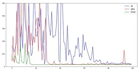
Figure 5:The steps amount in the #25 maze per episode comparison.The X axis is the episode number,and the Y axis represents the number of steps in each episode

Figure 6:The number of steps in the #908 maze per episode

All three algorithms are compared in terms of average exploration efficiency of each step in every episode when they are applied to solve all the mazes,and again,the results from mazes 25 and 908 are plotted in Fig.7 and Fig.8,respectively.One can see that SFW is more efficient in exploration and converges faster than the other two algorithms.

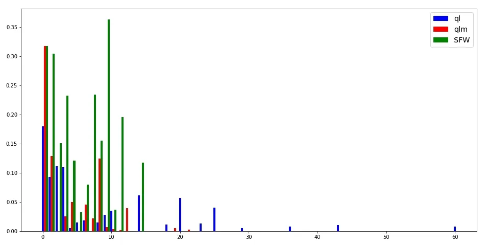
Figure 7:Average exploration efficiency while solving maze 25

5.2.2 Statistical performance comparisons for all mazes

The experiments in this section include all 975 mazes.The X axis of each figure corresponds to the maze number.

The comparison of convergence speed of every maze is shown in the Fig.9 and Fig.10,where ql and qlm are compared with SFW separately.The Y axis of each figure is the number of episodes when the agent for the first time arrives at convergence.In both figures,one can see that the proposed algorithm converge more quickly than the other two algorithms,especially true when there are a large number of episodes.Actually,the SFW alogirthm converges after no more than 20 episodes,while the other two algorithms need as many as 100+ episodes.

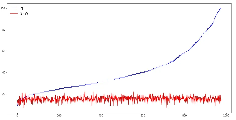
Figure 9:Convergence speed comparison:ql and SFW

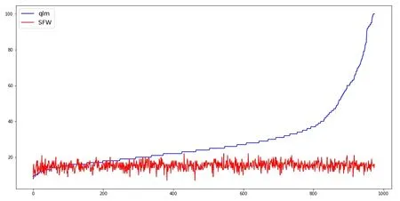
Figure 10:Convergence speed comparison:qlm and SFW

The lengths of the finally discovered paths by are reported in Fig.11 and Fig.12.One can see that the paths found by SFW have shorter lengths,in the range of 15 to 20,while the paths found by the other two algorithms are much longer.In quite a few cases,the paths found by ql and qlm are twice longer than those found by SFW.

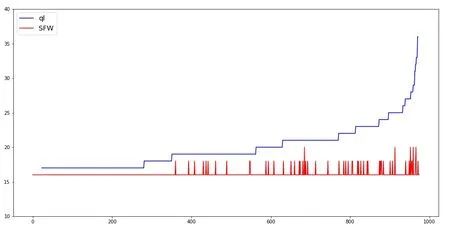
Figure 11:Steps length of convergence comparison:ql and SFW

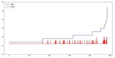
Figure 12:Steps length of convergence steps comparison:qlm and SFW

The exploration efficiency obtained from solving every maze is shown in Fig.13.One can see SFW outperforms qlm in this regard,and both algorithms are significantly better than ql.The X axis represents the maze number.The Y axis is the ratio of the total number of explored states to the total number of steps when the agent for the first time arrives at convergence.

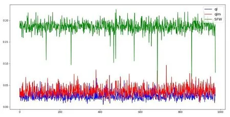
Figure 13:Explore efficiency comparison

5.3 The maze in the dynamic environment

Changes of environment are categorized as obstacle change and target position change.We will in this subsection examine how these changes can affect the performance of the three algorithms.

5.3.1 Obstacle change

Take Maze #8 as an example,the changes of the obstacles are tabulated in Tab.5.

Table 5:Dynamic obstacle,Maze #8

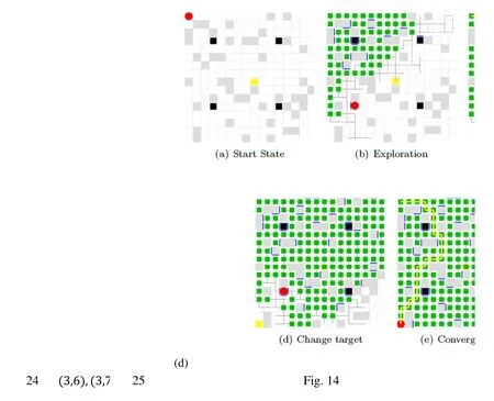
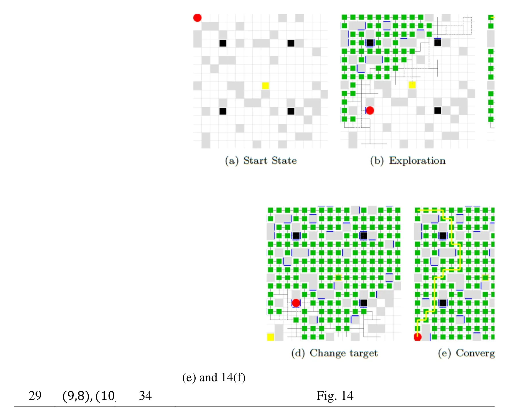
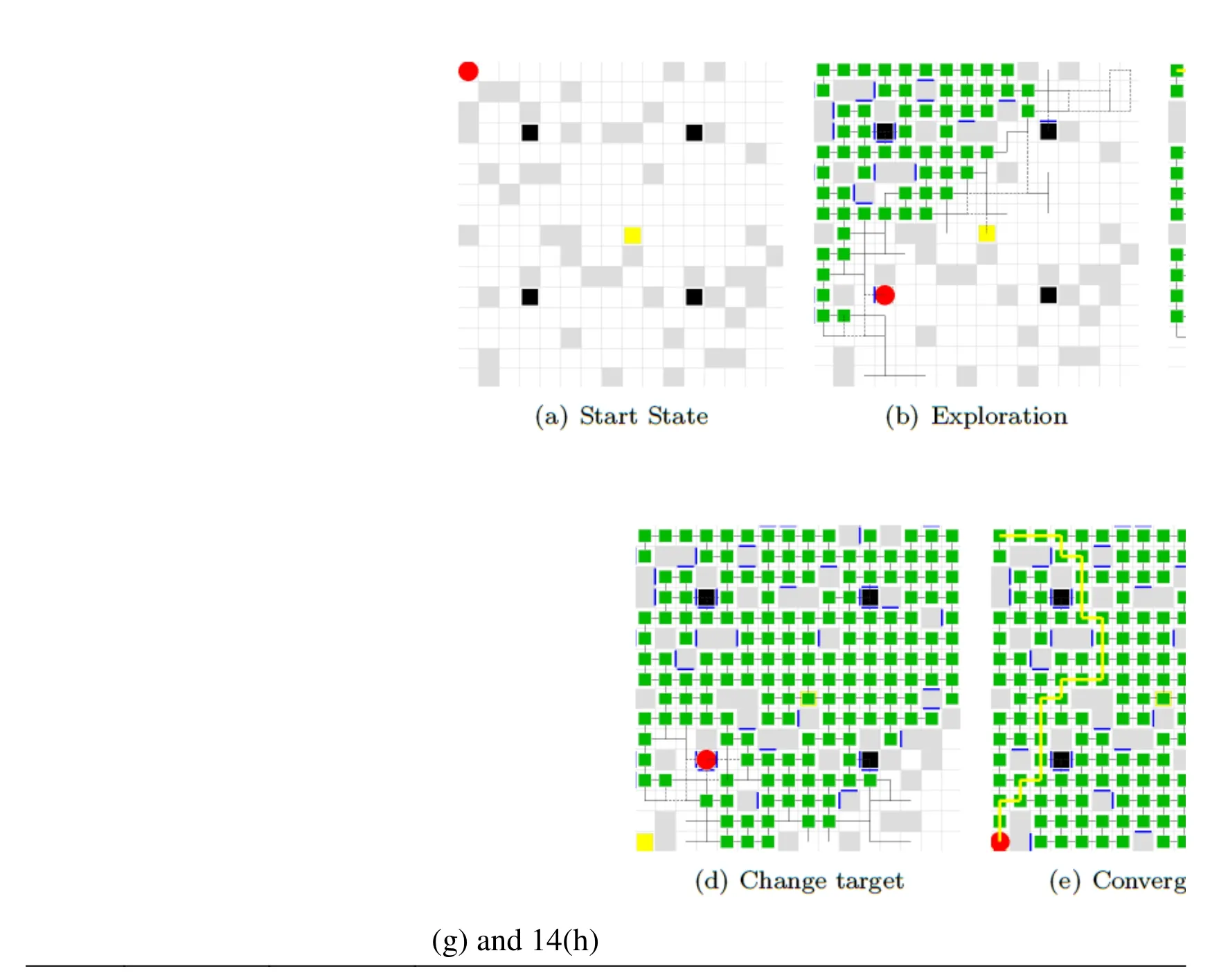
Fig.14 shows the snapshot of exploration,convergence,environment change and adaptation.The maze has undergone three major changes that occur to the locations of the obstacles in the experiments.The green squares in Fig.14 represent the members of SE,and the purple squares represent dynamically increased obstacles that are located within the current convergent path.

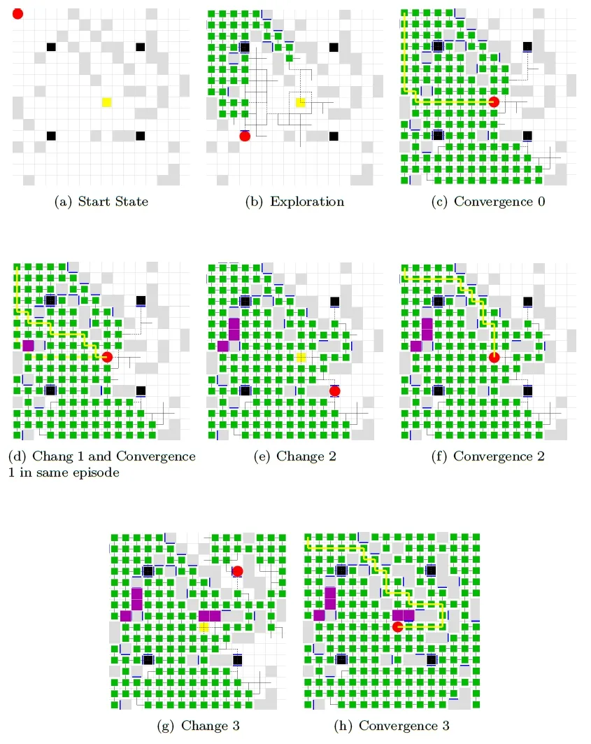
Figure 14:Dynamic obstacles,Maze #8

5.3.2 Changes of target positions

Tab.6 summarizes the changes that occur to maze 243.Other mazes have gone through similar changes.One can see that the target position is changed once,relocated from the center of the maze to its lower left corner.

Table 6:Dynamic target,Maze #243

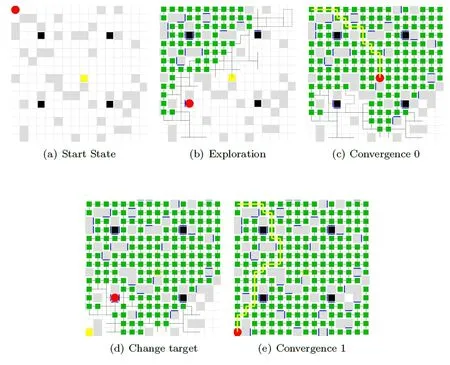
Figure 15:Dynamic target,Maze #243

The results of exploration,convergence due to target position changes and reconvergence are shown in Fig.15.In episode 0,the reward is claimed at block (9,9) (Fig.15(a)).The exploration converges in episode 14 (Fig.15(c)).In episode 18 where move the reward is moved to the block (1,16) (Fig.15(d)),the agent finds the right path to the target,after three episodes (Fig.15(e)).

5.4 Computation efficiency

All three algorithms are compared for their respective computation efficiency under the same computation platform.The hardware used in the experiments has a Intel(R) Core(TM) i5-3210M CPU running at 2.50 GHz,and a RAM size of 8 GB.The operating system is Ubuntu 64bits.The tools used to test CPU time and memory occupation are line_profiler and memory_profiler,respectively.

The average CPU time reported in Tab.7 is the average time of solving all 975 mazes.The basic memory usage in Tab.7 refers to the stable memory usage collected from solving select 62 mazes.One can see that SFW requires more memory space than the other two algorithms;the memory usage for both ql and qlm is comparable.The peak memory usage of SFW is also higher than that of ql or qlm.

Table 7:Algorithm complexity comparison

6 Conclusion

In this paper,a new graph-based method was presented for reinforcement learning.Unlike classical Q-learning algorithm and improved Q-learning algorithm,the proposed algorithm does not struggle with the exploration vs.exploitation tradeoff,as it was proved that the two tasks of exploration and exploitation actually converge in the decision-making process.As so,the proposed graph-based algorithm finds the shortest path during exploration,which gives higher efficiency and faster convergence than the Qlearning algorithm and its variant.Another big advantage of the proposed algorithm is that it can be applied to the dynamic environment where the value-oriented algorithm fails to work.The efficiency and convergence performance of the proposed algorithm comes at a cost of increased computational complexity.Future study will be focused to confine the computational complexity and particularly memory usage.

Acknowledgements:This research work is supported by Fujian Province Nature Science Foundation under Grant No.2018J01553.

The authors would like to thank the U.S.DOT Tier 1 University Transportation Center on Improving Rail Transportation Infrastructure Sustainability and Durability.

References

Dayan,P.;Hinton,G.E.(1993):Feudal reinforcement learning.Advances in Neural Information Processing Systems,pp.271-278.

Dietterich,T.G.(1998):The maxq method for hierarchical reinforcement learning.ICML,vol.98,pp.118-126.

Dijkstra,E.W.(1959):A note on two problems in connexion with graphs.Numerische Mathematik,vol.1,no.1,pp.269-271.

Floyd,R.W.(1962):Algorithm 97:shortest path.Communications of the ACM,vol.5,no.6,pp.345.

Hart,P.E.;Nilsson,N.J.;Raphael,B.(1968):A formal basis for the heuristic determination of minimum cost paths.IEEE Transactions on Systems Science and Cybernetics,vol.4,no.2,pp.100-107.

Huang,B.Q.;Cao,G.Y.;Guo,M.(2005):Reinforcement learning neural network to the problem of autonomous mobile robot obstacle avoidance.Proceedings of 2005 International Conference on Machine Learning and Cybernetics,vol.1,pp.85-89.

Kaelbling,L.P.;Littman,M.L.;Moore,A.W.(1996):Reinforcement learning:a survey.Journal of Artificial Intelligence Research,vol.4,pp.237-285.

Lewis,F.L.;Varbie,D.;Vamvoudakis,K.G.(2012):Reinforcement learning and feedback control:Using natural decision methods to design optimal adaptive controllers.IEEE Control Systems,vol.32,no.6,pp.76-105.

Lewis,F.L.;Varbie,D.(2009):Reinforcement learning and adaptive dynamic programming for feedback control.IEEE Circuits and Systems Magazine,vol.9,no.3,pp.32-50.

Mataric,M.J.(1997):Reinforcement learning in the multi-robot domain.Robot Colonies Springer Press,pp.73-83.

Moore,A.W.(1994):The parti-game algorithm for variable resolution reinforcement learning in multidimensional state-spaces.Advances in Neural Information Processing Systems,pp.711-718.

Smart,W.D.;Kaelbling,L.P.(2002):Effective reinforcement learning for mobile robots.IEEE International Conference on Robotics and Automation,vol.4,pp.3404-3410.

Sutton,R.S.;Barto,A.G.;Williams,R.J.(1992):Reinforcement learning is direct adaptive optimal control.IEEE Control Systems,vol.12,no.2,pp.19-22.

Silver,D.;Hubert,T.;Schrittwieser,J.;Antonoglou,I.;Lai,M.et al.(2017):Mastering chess and shogi by self-play with a general reinforcement learning algorithm.arXiv,preprintarXiv:1712.01815.

Silver,D.;Schrittwieser,J.;Simonyan,K.;Antonoglou,I.;Huang,A.et al.(2017):Mastering the game of go without human knowledge.Nature,vol.550,no.7676,pp.354-359.

Silver,D.;Huang,A.;Maddison,C.J.;Guez,A.;Sifre,L.et al.(2016):Mastering the game of go with deep neural networks and tree search.Nature,vol.529,no.7587,pp.484-489.

Sutton,R.S.;Barto,A.G.(2017):Reinforcement Learning:An Introduction.MIT Press.

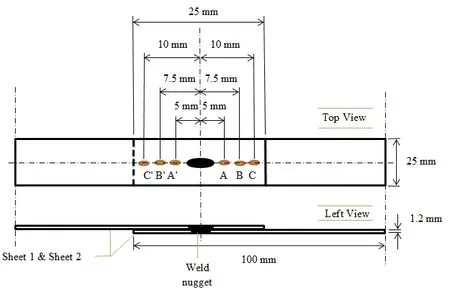
Figure 1:The located points on plate for X-ray diffraction measurements

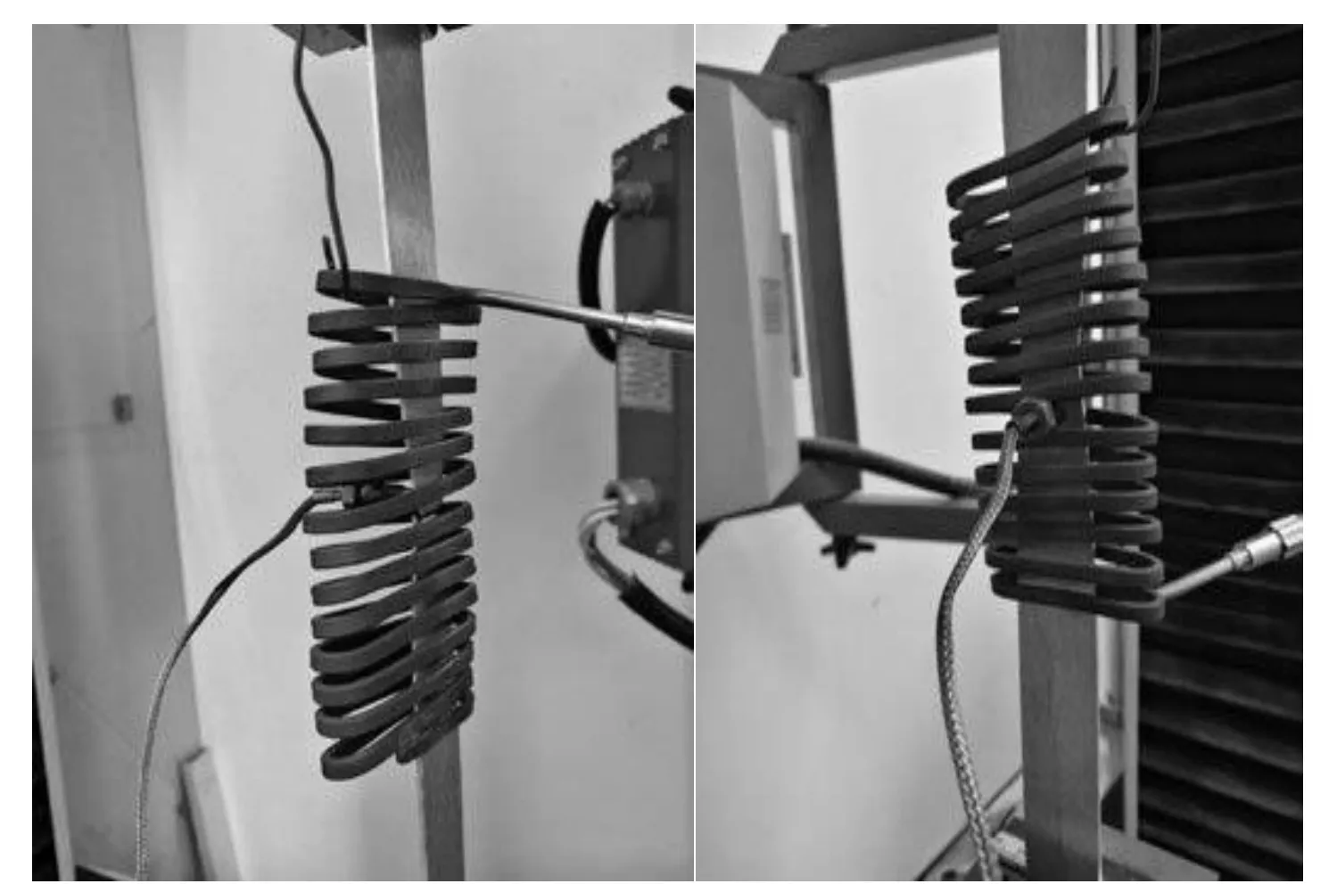
Figure 2:The temperature dependent tensile test

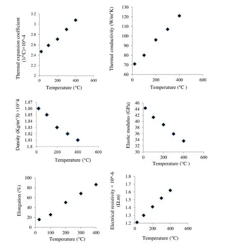
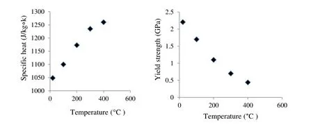
Figure 3:Experimentally determined thermophysical and thermomechanical properties of AZ61 Mg alloy

3 Finite element model

RSW exerts high temperature cycles on the welding structures because of its concentrated and localized heating nature.This process causes nonlinearities in mechanical behavior of the material,which makes it very difficult to be studied analytically.In fact,the analytic study of RSW contains many equations such as electrical,thermal,and structural that must be simplified to be solved,and this would cause significant errors in final results.For this reason,numerical techniques have been developed and adopted.The model geometry adopted in this work is shown in Fig.4.Due to the symmetric axis,one half of the sample considered for modeling.

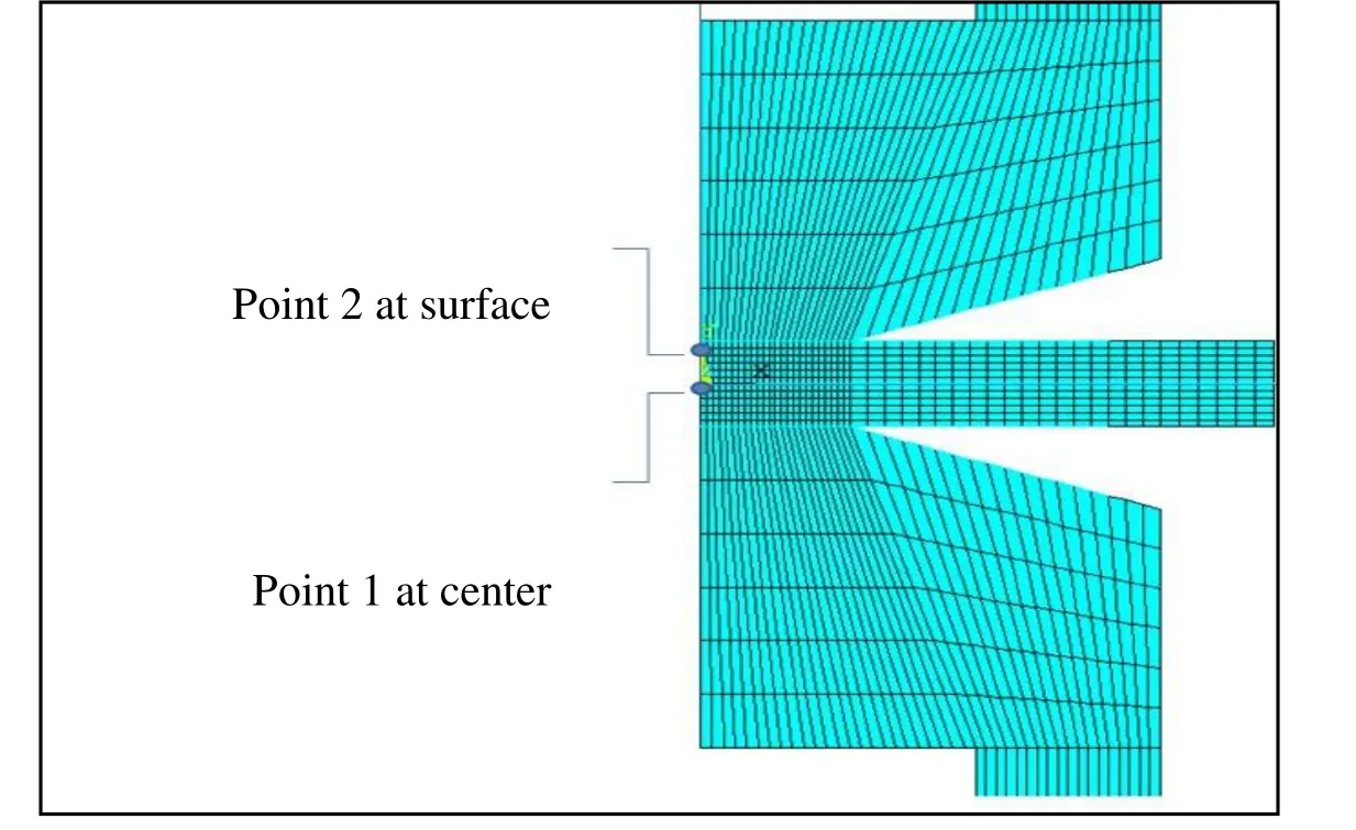
Figure 4:Axisymmetric FE model used in the calculations;points 1 and 2 are two points on the center of weld nugget and surface of sheet metal,respectively

Since the RSW process is a complex phenomenon involving thermal,electrical,and mechanical properties,an incremental fully-coupled mechanical-electrical-thermal FE model has been used in this study.Eq.(1) presents the governing equation for calculation of the thermal analysis:

Where,ρ is the materials density,Cis the heat capacity,Tis the temperature,Kis the thermal conductivity and(v) is the internal heat generation rate per unit volume.Based on the Fourier isotropic nonlinear relation of temperature density,thermal boundary conditions can be shown by Eq.(2):

And the equation for the surface boundary conditions is:

Where,qis the thermal flux on the surface andnis the external normal surfaces vector.The governing equation for the calculation of the electrical potential φ can be presented by Eq.(4):

Where,Ceis the electrical conductivity,ris the radial distance andzis the distance in the axis direction.The following matrix for coupling of the thermal and the electrical problems is:

Where,[Ct] is the special heat matrix,[Kt] is the thermal conductivity matrix,[Kv] is the electricity matrix,{T} is the temperature vector,{V} is the electrical potential vector,{Q} is the heat flux vector and {I} is the electrical current vector.Based on the equilibrium relation of the stress,the mechanical analysis can be shown by Eq.(6):

Where σ is the stress,bis the force andris the coordinate vector.And also the material properties equation based on the thermal-elastic-plastic theory is as follows:

Where,{σ} is the stress vector,[D] is the elastic-plastic matrix,{ε} is the strain vector,[De] is the elastic matrix and {α} is the thermal expansion coefficient.

In the FE model,the whole steps of RSW process have been considered including squeeze,welding,holding,and cooling.RSW begins with squeezing step,which is performed by mechanical FE model.Results of this step are deformation,contact pressure,and size of contact areas.These data have been considered as initial conditions for further welding cycle.In the welding cycle,a root mean square electrical current according to Eq.(9) has been uniformly applied at the top surface of the upper electrode.The electrical current reaches the bottom surface of the lower electrode where the voltage is zero after passing through the contact area between the electrode-sheet and sheet-sheet.

Wherefis the frequency andI,ImandIrmsare the real electrical current,the peak of the electrical current and the root mean square electrical current respectively.

The result of the electrothermal FE model is the temperature distribution.The temperature distribution has been used as a preload for thermomechanical FE model.The results of this FE model are deformations and the size of contact regions which have been reserved and utilized for the next increment of electrothermal FE model as an updated preload.The loop continues up to the end of welding time.At the holding cycle,pressure of the electrodes is sustained to form the nugget while the electrical current has been turned off.At the cooling step,the electrodes have been removed from the contact areas by birth and death element technique.In this step,sheets have been cooled down by convection to reach ambient temperature.The temperature gradient then causes residual stresses.At the end of all steps,the residual stress distribution can be extracted from the FE model.

The plane182 and plane67 element types have been utilized for mechanical and electrothermal analysis respectively.The Targe169 and Conta171 element types have been used to display contact areas on the electrode-workpiece interfaces and workpieceworkpiece faying surfaces.Temperature dependent electrical contact conductance (ECC) and thermal contact conductance (TCC) of copper electrode and magnesium AZ61 alloy have been used in contact area [Karimi,Sedighi and Afshari (2015)].Also,the imposed boundary conditions are presented in Fig.5.

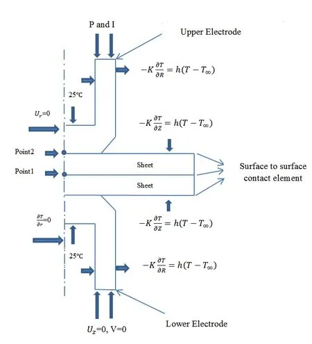
Figure 5:Imposed boundary condition on FE model

In the FE model,shape and size of the elements have important effect on the solution convergence.Mesh sensitivity analysis has been performed with different number of elements (with coarser up to finer elements).Fig.6 shows that the model with 732 elements is the optimum number of mesh because of no significant temperature change.

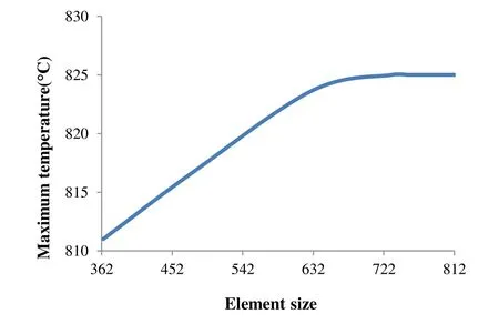
Figure 6:The mesh sensitivity diagram in electrothermal step (welding current:16 KA;welding time:16 cycles;electrode force:1130 N)

4.Results

First,the FE model has been validated by the experimental data obtained from the welding size and residual stresses measuring tests.As Fig.7 illustrates a good agreement has been detected between the nugget size and shape obtained from the experimental test and FE model.It is important to indicate that the melting point of AZ61 magnesium alloy supposed to be as 650°C and the nugget size has been obtained from the FE model at the end of welding cycle.So the negligible difference between the results occurs because of shrinkage in the experimental test when the nugget cools down to the ambient temperature.In addition,the measured residual stresses from XRD and predicted residual stresses from FE are presented in Tab.2.The results presented in this table confirm that the FE model has a good reliability to predict the residual stresses in RSW of AZ61 alloy.

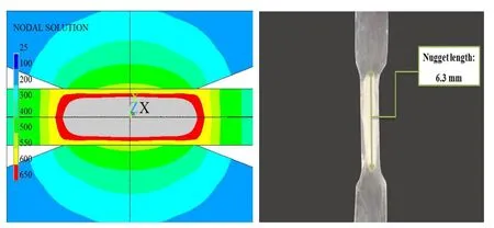
Figure 7:The comparison between FE model and experimental nugget size.

Table 2:Comparison of max principal residual stress obtained from experimental,FE model and the errors

Fig.8 shows the temperature and the longitudinal residual stress histories for two points:the center of weld nugget and the surface of sheet metal (Fig.4).In Fig.8a the maximum temperatures for both points have been reached the end of welding cycle,and they have been decreased down to the end of the holding cycle.Also,these points have equal magnitude and trend at the end of the cooling cycle.

The maximum longitudinal compressive residual stress has been occurred at the welding cycle,and also located at the center of nugget (Fig.8b).However,the compressive residual stresses reduce,the tensile residual stresses rise up while the time increases.

The temperature reaches to the maximum value at the end of the welding cycle,so the materials in fusion zone tend to expand.The major factors controlling this expansion are temperature and electrode force.The expansion is confronted by relatively cold surrounding materials and these interactions lead to compressive residual stresses.After the welding cycle,there is a decrease in magnitude of compressive residual stresses.At the holding cycle and also cooling cycle,the shrinkage occurs when the nugget cools down and this phenomenon is confronted by relatively cold surrounding materials and these interactions lead to tensile residual stresses as shown in Fig.8b.At the holding cycle copper electrodes have a significant effect on cooling rate as heat sinks.

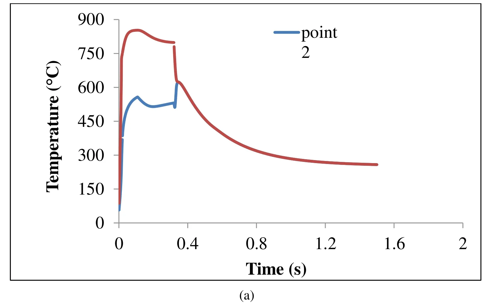
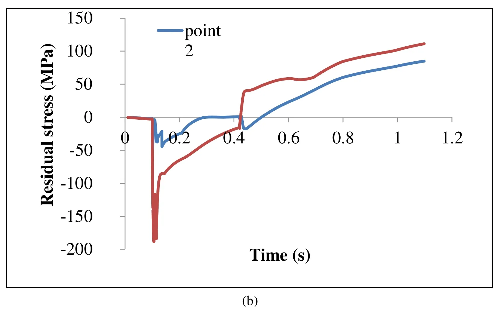
Figure 8:(a) Temperature histories and (b) Stress histories of point 1 (TEMP center,SX_center) and point 2 (TEMP_surface,SX_surface)

At the holding cycle,a high thermal gradient occurs between the sheet surface contacts and the other sheet regions.These regions,the top and the bottom of the sheet,have direct contact with the electrodes.So,they have been cooled very fast in comparison to the hottest region such as the weld nugget.This thermal gradient remains till the electrodes are removed.In this step,there is no contact between sheet and electrodes.Therefore,the temperature of the sheet surface contacts quickly increases while temperature in the weld area reduces.After holding cycle,the temperature of these points has equal magnitude and same trend.They fall down to the ambient temperature at the cooling cycle as shown in Fig.8a.

In spite of aluminum alloys,which different changes of residual stresses have been detected at center-line and surface-line [Ranjbar Nodeh,Serajzadeh and Kokabi (2008)];for magnesium alloys,reduction in both lines have been discovered as shown in Fig.8.Moreover,Fig.9 clearly shows that there is a reduction of residual stresses inside and outside of the nugget zone by moving to the end of the sheet.

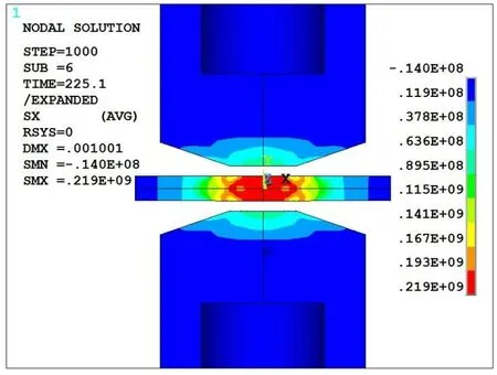
Figure 9:Residual stress distribution for sample 2

However,there are many influential parameters in RSW,in this study the effects of welding current,welding time,and electrode force have been investigated on the maximum tensile residual stress which arises at the center of nugget.Figs.10,11 and 12 present the effects of the welding time,welding current,and electrode force on the maximum tensile stress respectively.Fig.10 shows that the maximum tensile residual stresses are reduced by increasing the welding time.However by improving the welding time during the welding cycle the heat raises according to the Joule’s heat law,the produced heat in nugget transfers to the outside region more quickly.This heat transfer leads to a further decrease in the temperature gradient between the nugget and the surrounding regions which reduce the resultant residual stress.

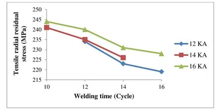
Figure 10:The effect of welding time on the maximum tensile residual stress (electrode force:848 N)

Fig.11 displays that the tensile residual stress in welded joints rises by improving the welding current.As the welding current increases,the heat produced in nugget rises,and thereby the gradient of temperature between nugget and its surroundings areas increases.Fig.12 illustrates that the maximum tensile residual stress declines by increasing the applied electrode force.Actually,increasing the electrode force subsequently raises the compressive stresses at the welded area.

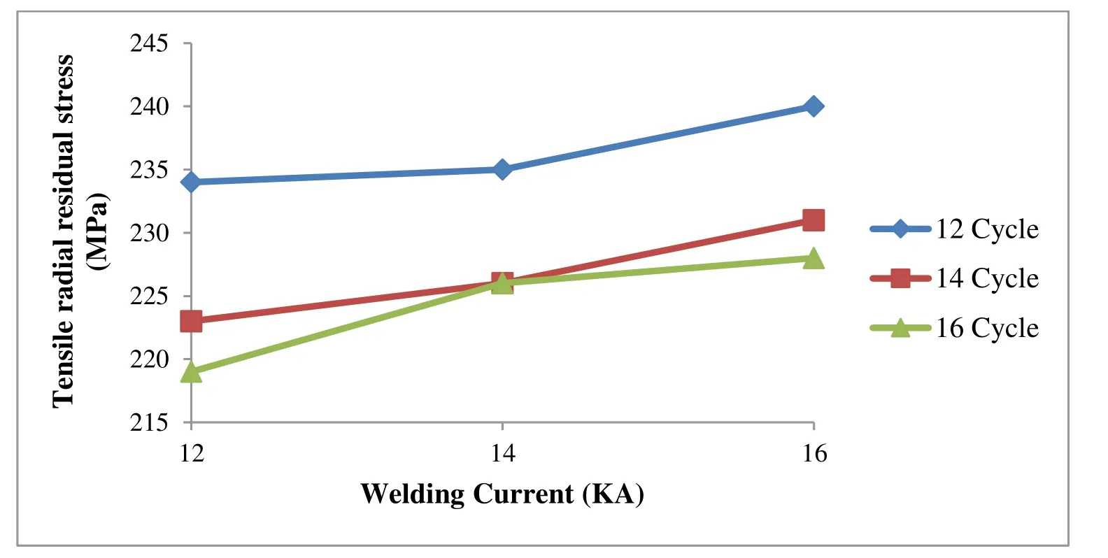
Figure 11:The effect of welding current on the maximum tensile residual stress (electrode force:848 N)

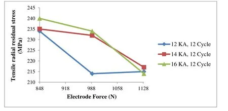
Figure 12:The effect of electrode force on the maximum tensile residual stress

5 Conclusion

In this study a structural-thermal-electrical FE model has been utilized to study the distribution of residual stresses in resistance spot welded AZ61 magnesium alloy sheet.

Also,the experimental measurements have been carried out by using XRD to validate the FE model.Moreover,the model has been utilized to investigate the effects of welding parameters such as welding current,welding time,and electrode force on the maximum tensile radial residual stress.The obtained results show that:

(1) The presented FE model is reliable to predict the nugget size and distribution of residual stresses occurred during the RSW process.There is a good agreement between the results obtained from the FE model and the experimental tests.

(2) While the maximum tensile residual stresses occurred in the nugget center,the reduction inside and outside of nugget zone are detected by moving to the end of the sheet.

(3) In order to decrease the tensile radial residual stresses in the welding area,an upper limit of welding time and electrode force are required while the welding current should be in its minimum level.

References

Afshari,D.;Sedighi,M.;Karimi,M.R.;Barsoum,Z.(2013):On residual stresses in resistance spot-welded aluminum alloy 6061-T6:experimental and numerical analysis.Journal of Materials Engineering Performance,vol.22,no.12,pp.3612-3619.

Asle Zaeem,M.;Nami,M.R.;Kadivan,M.H.(2007):Prediction of welding buckling distortion in thin wall aluminum T joint.Computational Material Science,vol.38,no.4,pp.588-594.

ASME(2002):Qualification Standard for Welding and Brazing Procedures,Welders,Brazers and Welding and Brazing Operators.ASME IX,American Society of Mechanical Engineers.

Barsoum,Z.(2013):Residual stress prediction and relaxation in welded tubular joint.Welding World,vol.51,pp.23-30.

Cha,B.W.;Na,S.J.(2003):A study on the relationship between welding conditions and residual stress of resistance spot welded 304-type stainless steels.Journal of Manufacturing Systems,vol.22,no.3,pp.181-189.

Florea,R.S.;Hubbard,C.R.;Solanki,K.N.;Bammann,D.J.;Whittington,W.R.et al.(2012):Quantifying residual stresses in resistance spot welding of 6061-T6 aluminum alloy sheets via neutron diffraction measurements.Journal of Materials Processing Technology,vol.212,no.11,pp.2358-2370.

James,M.N.;Webster,P.J.;Hughes,D.J.;Chen,Z.;Ratel,N.et al.(2006):Correlating weld process conditions,residual strain and stress,micro structure and mechanical properties for high strength steel-the role of diffraction strain scanning.Material Science Engineering,vol.427,no.1-2,pp.16-26.

Karimi,M.R.;Sedighi,M.;Afshari,D.(2015):Thermal contact conductance effect in modeling of resistance spot welding process of aluminum alloy 6061-T6.InternationalJournal of Advanced Manufacturing Technology,vol.77,pp.885-895.

Kramar,T.;Vondrous,P.;Kolarikava,M.(2015):Resistance spot welding of magnesium alloy AZ61.Modern Machinery Science,no.1,pp.596-599.

Manladan,S.M.;Yusof,E.;Ramesh,S.;Fadzil,M.(2016):A review on resistance spot welding of magnesium alloys.International Journal of Advanced Manufacturing Technology,vol.86,no.5-8,pp.1805-1825.

Moharrami,R.;Hemmati,B.(2017):Numerical stress analysis in resistance spotwelded nugget due to post-weld shear loading.Journal of Manufacturing Processing,vol.27,pp.284-290.

Moshayedi,H.;Sattari-far,I.(2014):Resistance spot welding and the effects of welding time and current on residual stresses.Journal of Materials Processing Technology,vol.214,no.11,pp.2542-2552.

Pakkanen,J.;Vallant,R.;Kiein,M.(2016):Experimental investigation and numerical simulation of resistance spot welding for residual stress evaluation of DP1000 steel.Welding World,vol.60,no.3,pp.393-402.

Parmar,R.S.(1999):Welding Processes and Technology.2nd ed.,Khanna Publishers,India.

Ranjbar Nodeh,I.;Serajzadeh,S.;Kokabi,A.H.(2008):Simulation of welding residual stresses in resistance spot welding,FE modeling and x-ray verification.Journal of Materials Processing Technology,vol.205,no.1-3,pp.60-69.

Satonaka,S.;Lwamoto,C.;Matsumoto,Y.;Murakami,G.I.(2012):Resistance spot welding of magnesium alloy sheets with cover plates.Welding World,vol.56,no.7-8,pp.44-50.