A Novel Ensemble Learning Algorithm Based on D-S Evidence Theory for IoT Security

Changting Shi

1 College of Computer Science and Technology,Harbin Engineering University,Harbin,150001,China

Abstract:In the last decade,IoT has been widely used in smart cities,autonomous driving and Industry 4.0,which lead to improve efficiency,reliability,security and economic benefits.However,with the rapid development of new technologies,such as cognitive communication,cloud computing,quantum computing and big data,the IoT security is being confronted with a series of new threats and challenges.IoT device identification via Radio Frequency Fingerprinting(RFF)extracting from radio signals is a physical-layer method for IoT security.In physical-layer,RFF is a unique characteristic of IoT device themselves,which can difficultly be tampered.Just as people’s unique fingerprinting,different IoT devices exhibit different RFF which can be used for identification and authentication.In this paper,the structure of IoT device identification is proposed,the key technologies such as signal detection,RFF extraction,and classification model is discussed.Especially,based on the random forest and Dempster-Shafer evidence algorithm,a novel ensemble learning algorithm is proposed.Through theoretical modeling and experimental verification,the reliability and differentiability of RFF are extracted and verified,the classification result is shown under the real IoT device environments.

Keywords:IoT security,physical-layer security,radio frequency fingerprinting,random Forest,evidence theory.

1 Introduction

The Internet of Things(IoT)is an important and advanced communication method in the 21stcentury [Atzori,Iera and Morabito(2010)].In the IoT environment,it allows the perception and control of physical objects through some basic network facilities,enabling integration between the computer system and the physical world.In recent years,sensors,actuators and mobile devices have appeared more and more frequently in our daily lives[Shi,Li,Zhu et al.(2018)].Because of its powerful communications and computing capabilities,the Internet of Things has covered all aspects of our lives [Lin,Yu,Zhang et al.(2017); Alvear,Calafate,Cano et al.(2018); Stankovic(2014); Al-Fuqaha,Guizani,Mohammadi et al.(2015)].In the IoT environment,seamless interaction between different kinds of equipment,such as vehicles [Lu,Cheng,Zhang et al.(2014)],medical sensors [He and Zeadally(2015)],monitoring location [Chen,Yang and Wang(2016)],cognitive communication appliances Yang et al.[Yang,Liu,Sun et al.(2017); Ding,Wang,Wu et al.(2015); Jia,Gu,Guo et al.(2016)] have resulted in the emergence of many applications,such as the emergence of smart cities [Alvear,Calafate,Cano et al.(2018)],home automation [Pirbhulal,Zhang,Me et al.(2017)],smart grid [Zaballos,Navarro and Martín(2018)],traffic management [Leone,Moroni,Pieri et al.(2017)] etc.As is well known,IoT will lead to improve efficiency,reliability,security and economic benefits in our daily life [Lee and Lee(2015)].

As we enter the IoT era in which the communication network is becoming increasingly dynamic,heterogeneous,and complex,a lot of new technologies such as cognitive communication,cloud computing,quantum computing and big data have been proposed,the IoT security is being confronted with a series of new threats and challenges [Lin,Yu,Zhang et al.(2017); Mpitziopoulos,Gavalas,Κonstantopoulos et al.(2009); Liu,Dong,Ota et al.(2017)].Since the IoT security protection strategy is still at a low level,many existing IoT networks cannot resist large amounts of malicious attacks now [Wu and Wang(2018); Cao,Shila,Cheng et al.(2016); Vasserman and Hopper(2013)],because IoT devices can be accessed from any location by commissioning the network.However,IoT security is more important than traditional networks because attackers may have the opportunity to control and destroy critical infrastructure.Therefore,it is very important to research and propose a new security strategy that is suitable for Internet of Things to fight against various attacks.

The identification and authentication IoT device based on radio frequency fingerprinting(RFF)is one of the most important physical-layer method for IoT security [Danev,Zanetti and Capkun(2012); Gungor and Κoksal(2016); Wang,Sun,Piao et al.(2016)],which have been widely used in intrusion detection [Hall(2004)],access control [Ureten and Serinken(2007)],wormhole detection [Rasmussen and Capkun(2006)],cloning detection [Danev,Heydt-Benjamin and Čapkun(2010)].RFF is extracted from radio signals from IoT devices,which is unique characteristic of IoT device themselves and can difficultly be tampered.In physical-layer,RFF is Just as people’s unique fingerprinting,different IoT devices exhibit different RFF which can be used for identification and authentication.As is well known,RFF is derived hardware imperfection of IoT device,which can be observed and extracted.New method about RFF has been put forward continuously in recent years.Ma et al.[Ma,Qian,Li et al.(2013)] proposed the GenePlayer,UHF passive tag physical layer identification system.GenePrint's accuracy for passive tag identification can be higher than 99.68%.Moreover,GenePrint can effectively defend against serious functional replay attacks.Huang et al.[Huang,Yuan,Wang et al.(2016)] proposed a novel specific emitter identification(SEI)method based on nonlinear dynamics and extracted permutation entropy as the signal's RF fingerprint to identify the emitter.In order to verify the performance of this method,bispectrum-based techniques and spurious-based techniques were compared.For wireless network cards,the proposed method works better than the bispectrum-based technique and the strayparameter-based technique.Applying the proposed method to a digital radio,it is found that this method has a classification accuracy that is extremely similar to the bispectrumbased technology and the spurious parameter-based technology.Security measures based on the PHY and statistical features extracted from the time domain(TD)have also been extensively studied in recent years.Lopez et al.[Lopez,Liefer,Busho et al.(2018)] used multi-discriminant analysis,the Maximum Likelihood and Random Forest(RndF)classifier to process temporal(TD)and Slope-Based FSΚ(SB-FSΚ)fingerprinting.The results show that for 12 different categories of equipment,where each manufacturer has two devices at two different set points,both classifiers are reliably implemented and the average cross-class percentage correct rate can be obtained.Reising et al.[Reising,Temple and Jackson(2015)] verified the benefit of Dimensional Reduction Analysis(DRA)and the performance of rogue equipment using discrete Gabor transform features.Followed this paper Bihl et al.[Bihl,Bauer and Temple(2017)] compared the performance of six DRA methods.Their experiments collected ZigBee radiation and compared the ZigBee device's classification and ID verification performance on a fullsize dataset.The results show that their proposed MLF method is superior to competitive methods.Wang et al.[Wang,Sun,Piao et al.(2016)] studied the reliability and differentiability of WPLI technology,and it is not clear whether the existing WPLI technology is applicable to the actual situation.They found that the existing WPLI technology did not meet the qualified precision in the actual scene,which stimulated the birth of the better RFFs.Jia et al.[Jia,Ma and Gan(2017)] attempted to improve the effect of radiation measurement recognition by using the method of the regular term that imposes the minimum prediction error.After applying this method to the actual data set,the results show that this method has excellent recognition rate and anti-noise performance.

In this paper,the structure of IoT device identification is proposed,firstly,the key technologies such as signal detection,RFF extraction,and classification model is discussed.Secondly,based on the random forest and Dempster-Shafer evidence algorithm,a novel ensemble learning algorithm is proposed.Finally,the author completed modeling and verification of RFF,evaluated the reliability and differentiability of the method,and displayed the classification results in a real IoT device environment.Finally,the advantages and disadvantages of the proposed algorithm and its future prospects are described.

2 General view

In Fig.1,the physical-layer device identification system includes following parts:A signal collecting device for acquiring signals from the identified device; a burst extraction module to detect the begin of the turn-on transient and intercept it; a signal analysis module for obtaining relevant information from the signal; a fingerprint generation module to reduce assist information and generating the Radio Frequency Fingerprints(RFF); and a classifier to compare RFF and notify the system to identify the results [Patel,Temple and Baldwin(2015); Κlein,Temple,Mendenhall et al.(2009)].Other than that,to better verify the capability of this device at different signal-to-noise ratio,we add the Additive White Gaussian Noise(AWGN)module and the data condition module.Each part of the algorithm involved in this paper is shown on the right side of the Fig.1.

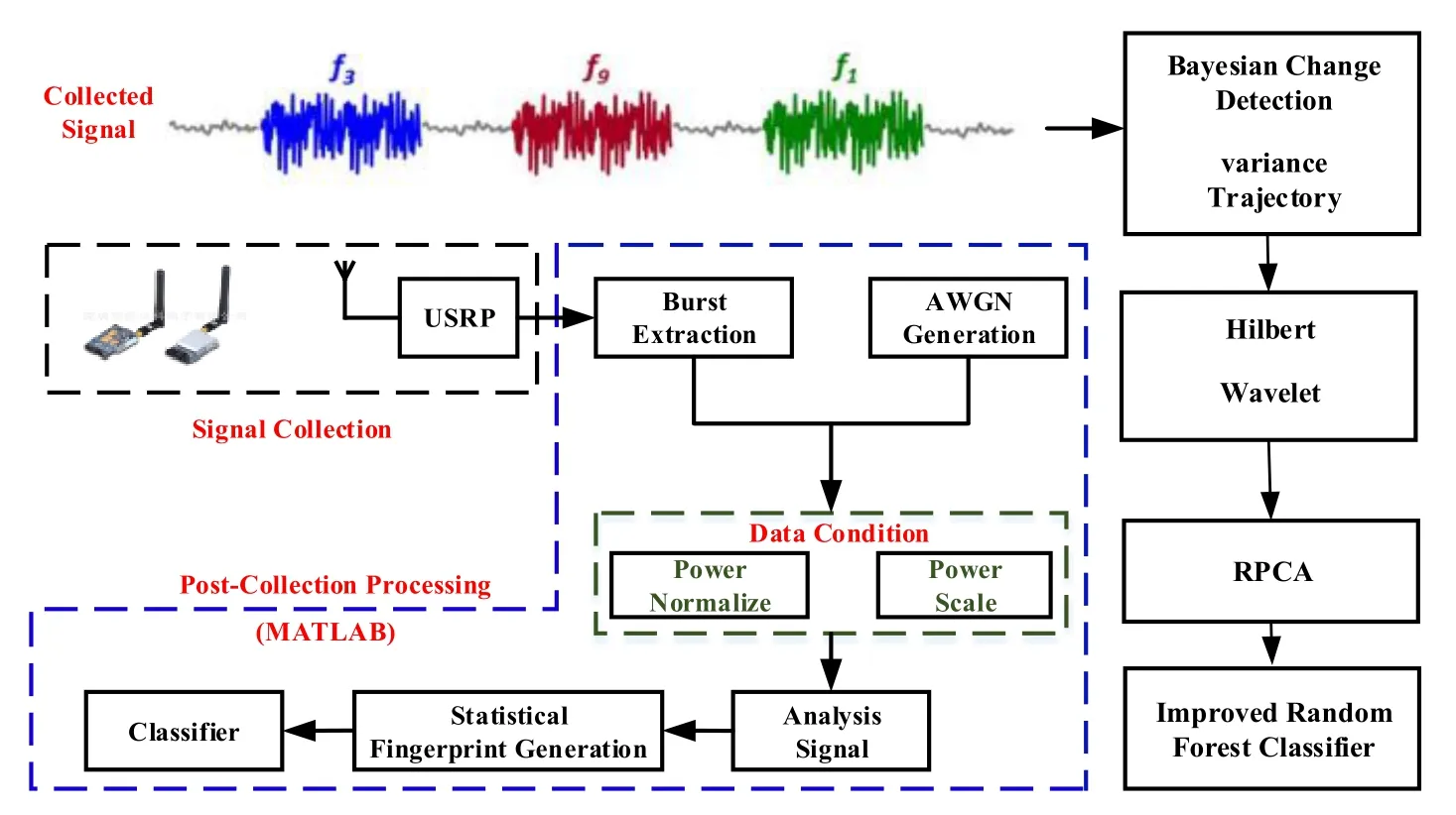
Figure 1:IoT device identification process

2.1 Data set definitions

The instantaneous RF signal is transmitted through 10 IoT devices.The device that collects the signals is the Agilent receiver.In order to eliminate noise during signal collection,we directly connected the IoT equipment to a spectrum analyzer.The noise in the following experiment was generated by software simulation.

Figure 2:The scheme of signal collection

The original data set contains 500 turn-on transient signals from 10 IoT devices.Each of these devices generates 50 noise-free transients,and the original data set is sampled by authorized devices.Of all the transient signals,300 constitute the training data set and another 200 make up the test data set.Artificially added Gaussian white noise after signal acquisition,the signal to noise ratio ranges from 0 dB to 20 dB(stepping to 2.5 dB).

2.2 Signal collection methodology

Transient extraction is very necessary in fingerprint identification.Because the problem is extracted instantaneously,the RF fingerprint cannot effectively express the characteristics of the signal.In this paper,the Variance Trajectory(VT)algorithm and Bayesian Change Detection(BCD)algorithm are used to detect transient signal.

2.2.1 Variance trajectory detection

The VT sequence ｛VTx(i)｝use the amplitude of the received signal ｛x(k)｝,k=1,2,...,Nxto detect the change point of transient signal.The ithelement of ｛VTx(i)｝can be calculated as [Ii,Temple,Mendenhall et al.(2008)]:

where,Nwis the number of sample point in the slipped-window,and Nsis the Step values between adjacent windows.The μwis the mean of ｛xw(k)｝,which is the subsequence of signals ｛x(k)｝intercepted by the window function.

2.2.2 Detection bayesian change detection

The BCD algorithm is more effective for signal with the power increase slowly.This kind of signal can be simplified as:

where d is a Ν×1matrix of original sample and e is a Ν×1matrix of Gaussian noise sample,G is of size N M .Each column of Gis a basis function evaluated at each point in the time series and each element of the M 1matrix bis a linear coefficient.The posteriori probability density can be calculated as follow [Ii,Temple,Mendenhall et al.(2008)]:

where I refers to the signal model defined in Eq.(3).The location of the change point is included in the matrix G and for a ramp change:

It is the main advantage of this method that no prior knowledge is required for obtaining probability density.The position of the maximum a posteriori probability is the location of the transient point.Fig.3 shows the turn-on transient signal of different IoT devices introduced in Section 2.1.

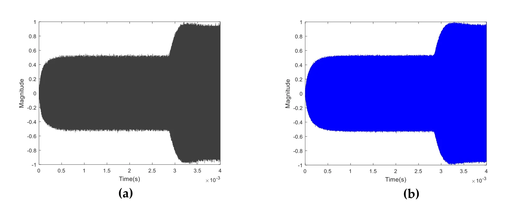
Figure 3:The turn-on transient signal of IoT device,(a)Device 1#;(b)Device 5#

It can be seen from the turn-on transient signal in Fig.3 that the signals under identification are almost similarity,it is difficult to distinguish it from the conventional method.Therefore,the more effective feature extraction and classification algorithm is of great significance for the identification process.

2.3 Signal analysis

Hilbert transform is a commonly used signal processing algorithm.Through the Hilbert transform,we can get the analytic form of the original signal,which can be used to calculate the instantaneous amplitude,phase and frequency of the signal.

Given a real-time time signal x(n),the Hilbert transform of this signal can be defined as follows:

It can be learned from the formula thatˆ(n)and x(n)are linear correlation.The phase of the original signal will appear j(π /2)after the transformation.The signal after the transformation is the harmonic conjugate of the original signal x(n)[Atzori,Iera and Morabito(2010)],from this method a real signal can be transform to its analytic form.Meanwhile we can calculate the instantaneous amplitude as follow:

Because of the transient signal captured in Section 2.1 have a long time length,the memory requirements for the subsequent processing will be very high.In order to reduce the number of sampling points,at the same time,retain the original information as far as possible.We extract the original sampled signals,and the number of sampling points per signal sample is 3187.Fig.4 is the instantaneous envelope carve of an IoT device extracted from transient signal.

Figure 4:Hilbert transform envelope of transient signal

2.4 Fingerprint generation

The classical Principal Component Analysis(PCA)is one of the most classical algorithms for high dimensional data processing.The algorithm criterion of PCA is the minimum mean square error.The Robust Principal Component Analysis(RPCA)is the improved method of PCA through a matrix decomposition.For a matrix M ∈ R(n1×n2),RPCA will decompose it into a low-rank matrix L ∈ R(n1×n2),which is the same size as the original matrix,and a sparse matrix S.Sparse matrix can be computed by solving the convex optimization as follow [Van Trees and Bell(2009)]:

For verifying the performance of the former algorithm,the dataset in Section 2.1 is used for simulation.RPCA is used for dimension reduction.According to the energy ratio of different dimensions,the first two are selected for visualization.

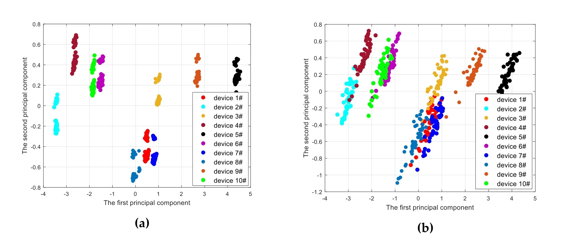
Figure 5:Two-dimensional principal components of 10 IoT devices’subtle features under different environment,(a)high SNR(≥50);(b)SNR=20 dB

From Fig.5,we can see that characteristics can achieve good separation between different signals at higher SNR conditions.The performance will decrease at low SNR,but it still can achieve the separation of different signal categories.For better verifying the performance of the ensemble learning classifier proposed in this paper,the Hilbert instantaneous amplitude envelope feature extraction method is used in the following experiment.

3 Designed classifier

Random forest classifier is an effective classification method.However,this method does not take into account the differences between different classifiers in the process of voting decision.In order to get more accurate classification results,we combine different probability of different sub-classifiers,and the evidence theory is performed on the identification results of random forest sub-classifiers placed at different positions.

3.1 Random forest

Random Forest is a classifier fusion algorithm proposed by Breiman [Breiman(2001)] in 2001.It is an ensemble classifier composed of multiple decision trees.Multiple decision trees are trained and all decision trees at the output vote for the results.It has a good performance in the classification of high-dimensional features [Κulkarni and Sinha(2012); Κumar,Κuppusamy and Aghila(2018)].Compared with the single classifier,the random forest classifier has higher accuracy and it also has better robustness for the noise data.

Random forests are very suitable for solving the problem of multi-classification task.Several decision trees ｛h(x,θk),k=1,2,...,ntree｝ can be used together for decision.Each classifier h(x,θk)is a decision tree without pruning,which has the advantages of fast and efficient [Patel,Temple and Baldwin(2015)].

The random forest algorithm flow is as follows:

1.From the original data samples,N1tree subsample sets are selected with replacement method,and each subsample set is called sample subspace,which is used as a training sample set of a decision tree.

2.For each sample subspace,different from the split criterion of the traditional decision tree,M features of each decision tree node are selected randomly as the feature subspace,from which the optimal splitting attribute selection is then performed.

All the N tree decision trees vote on the test sample set to get the final output.

3.The flow diagram of the random forest is as Fig.6.

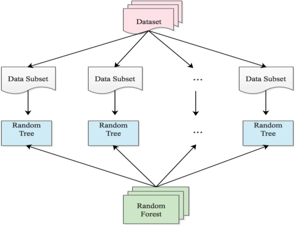
Figure 6:Random forest structure diagram

Random forests have a high generalization performance and different from the neural networks the over-fitted will not appear.It is mainly because of the two“random”concepts in the construction of random forests.One of them is to select subsets of samples by randomly placing back(bootstrap)during the generation of sample subspaces.The other is to randomly select features for each node during the generation of feature subspaces to split.In general,there is an empirical formula for the number of the selected feature.

where d is number of original features.It avoids the occurrence of the same or similar conditions in many decision trees.

When generating a random sample subspace,since all samples are randomly selected,there are some samples have not been sampled from beginning to end.These samples account for about 36.8% of the total sample,which are called out-of-pocket samples.Out-of-pocket samples can be used to estimate the importance of features [Nesa and Banerjee(2017)].

3.2 The background of dempster-shafer evidence theory

D-S evidence theory is an imprecise reasoning theory developed and perfected by Dempster and Shafer.It can solve some uncertain problems efficiently [Wang,Guo,Wang et al.(2017)].For a better understanding,some basic concept of this theory is follows.

Definition 1:Frame of Discernment(FD)

Firstly,a finite,nonempty,and exhaustive set Θ=｛F1,F2,,Fn｝is defined as frame of discernment,which contains all possible hypotheses of Fi and each hypothesis of Θis exclusive.

Definition 2:Basic Probability Assignment(BPA)

Suppose,each Fi is mapping to a number m(Fi)(m(Fi)∈[0,1]),the following requirement needs to be satisfied:

where,m(⋅)is the BPA on Ω(Θ),which shows the support degree of Fi.

For example,BPA can be shown as:m(F1)= 0.7,m(F2)= 0.2,m(F1,F2)= 0.1.It means that if ｛F1｝,｛F2｝,｛F1,F2｝happen,the respective support degrees corresponding to 0.7,0.2,0.1.

Definition 3:Focal Element(FE)

As it is defined in BPA,if m(Fi)＞ 0,Fi⊆Θ,then Fi is the focal element.For the example introduced former,the focal elements are ｛F1｝,｛F2｝,｛F1,F2｝.

Definition 4:Dempster’s Combination Rule(DCR)

Based on the same FD,BPA can be generated from different sensors,and those BPA can be combined via orthogonal sum,which is named as DCR.

3.3 A novel ensemble learning random forest based on evidence theory

As mentioned earlier,the final result of random forests is the result of voting by all decision trees.Traditional random forests simply use the minority to the majority to get the final category.However,this voting method does not take into account the differences between strong classifiers and weak classifiers.Once the number of decision trees giving wrong results is larger than the number of decision trees for correct classification results,the identification result of the entire random forest classifier is wrong.

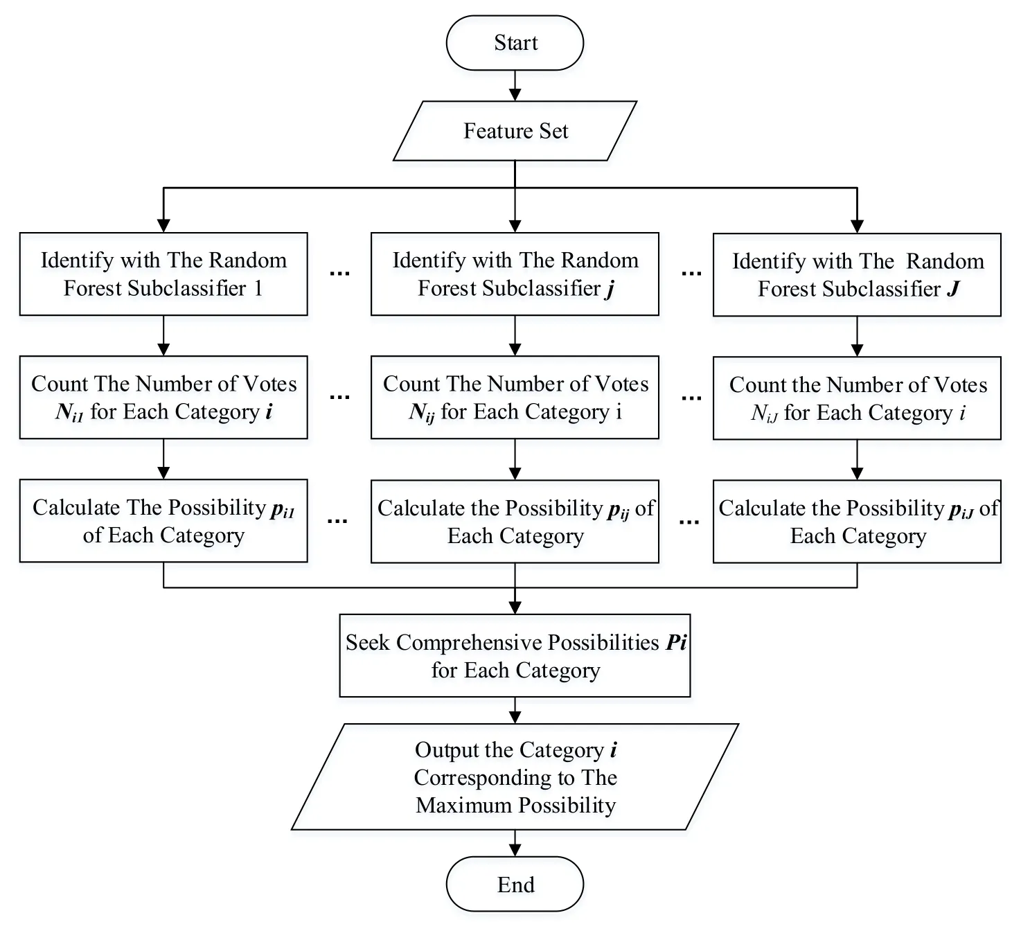
Figure 7:Flow chart of the ensemble learning random forest identification algorithm

For this reason,we can consider not voting for the moment in the output links but assigning a probability value to each category.In the form of probability.This possibility value is used as the basic probability assignment in the evidence theory,and the evidence combination is performed on the identification results of random forest sub-classifiers placed at different positions.The category with the highest probability of fusion is selected as the final category to improve the classification result.

The ensemble learning random forest algorithm is used in the identification process.The algorithm flow chart is shown in Fig.7.The algorithm flow with pseudo code is as follows:

Train J random forest sub classifiers,each sub classifier can be used as an independent random forest classifier.

Input the test sample to be identified xinto each sub classifier for identification.For therandom forest sub-classifier,record the test samples identification results of each test tree,and count the number of votes Nijfor each category i ,where i∈ ｛1,,I｝is the total number of categories.The possibility of the sample belongs to category iis pij:

Take the pijas the basic probability assignment,use the evidence theory to synthesize the output result pijof all Jsub-classifiers,get the corresponding post synthetic probability value pifor each category,and select the category with the maximum comprehensive probability value as the final output of the random forest.

When the data samples are covered with strong noise,a single random forest may lead to a wrong identification result.But the evidence theory combines multiple random forests as sub-classifiers,which can reduce the impact of the single classifier error decision,thus improve the accuracy of random forest identification.

4 Simulation result

4.1 Identification results under different dimensions

In this paper,the Hilbert transform is used to extract the unique feature for creating the fingerprinting.Then,we use Robust Principal Component Analysis(RPCA)to extract features form the original feature.

Figure 8:The change curve of the energy ratio with the dimensions

Fig.8 shows change curve of the energy ratio with the dimensions when using the RPCA method to reduce the dimension.The energy ratio refers to the ratio of useful information of feature vectors after dimensionality reduction to the useful information of the undiminished feature vector,which is calculated by the eigenvalues of the sample covariance matrix.The lower the dimensionality is,the less useful information it carries.Tab.1 shows the dimension after dimensionality reduction when the energy ratio of the original features 80%,85%,90% and 95% are respectively.According to the dimension corresponding to the typical energy ratio,in the rest of the paper,2 dimensional,76 dimensional,300 dimensional,and 645 dimensional samples are used for classification respectively.

Table 1:The dimension corresponding to the typical energy ratio

Fig.9 shows the variation in identification rate with different dimensions using random forest classifier.As the signal-to-noise ratio increases,the identification rate increases.When the input features have different dimensions,the classifier performs differently.In the range of 0 dB to 20 dB,the identification rate is always the highest when the dimension is 76,that is,the reduced dimension energy reaches 85%.When the 76-dimensional sample is selected as the input,the identification rate of random forest classifiers can achieve over 90% in the case where the SNR is greater than 10 dB.

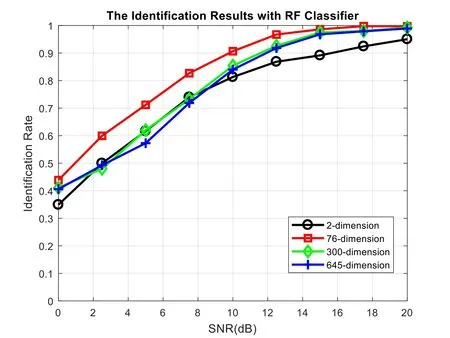
Figure 9:Identification rate of 10 IoT devices using random forest classifier

By observing the change of the identification rate with the input dimension,we can conclude that the identification rate increases first and then it will decrease with the increase of the dimension.The reason is that when the input dimension is too low,the device information carried by the feature is too small,and when the input dimension is too high,although the device information is more,this will increase the complexity of the classifier and also increase the number of redundancy.

4.2 A Novel ensemble learning classifier

Considering the simulation of Section 4.1,this paper chose to use the RPCA method to reduce the feature to 76-dimensions and use a random forest classifier as a comparative test.We put the ensemble learning random forest sub-classifiers around the IoT devices,the ensemble learning fusion classifiers based on evidence theory are used to obtain the final result from multiple sub-classifiers.

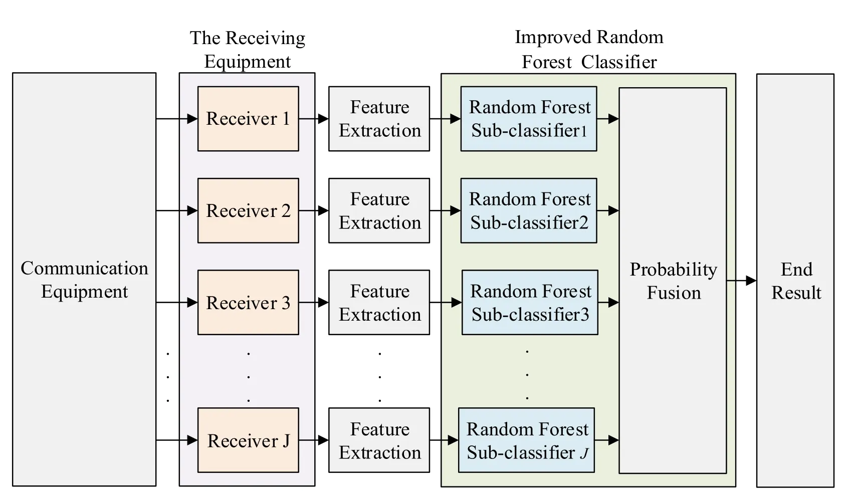
Figure 10:Structure diagram of ensemble learning random forest classifiers

In this experiment,every J test sample from the same device and SNR are used as an input of the ensemble learning random forest to simulate the performance of multiple sub-classifiers.Fig.11 is the identification rate of the D-S combination rule based(different number of sub-classifiers)and traditional rand forests(1 sub-classifier).

In order to compare the performance of the four combination rules,we get the identification rates with five sub-classifiers.We can see from Fig.11 that the number of sub-classifiers can make a difference in identification rate.When the number of subclassifiers 2,3,4 and 5 are compared with the traditional random forest classifier,the identification rate under low SNR increased significantly.The identification rate of the ensemble learning classifier is get a 22.3% improved compared with the traditional random forest classifier at 0 dB.Moreover,the greater the number of sub-classifiers,the higher the identification rate,which shows that the process of sub-classifier combination can effectively improve the accuracy of the classification.

Figure 11:Identification rate of traditional rand forest and ensemble learning rand forest with 4 combination rules

5 Conclusion

In this paper,we proposed a novel ensemble learning random forests classifier based on the D-S evidence theory.Ten Motorola interphones are used to verify the algorithm’s performance and make a comparison with traditional random forest algorithms.With the DS combination rule,the identification rate of ensemble learning random forest classifier got a 22.3% at 0 dB.Simulation result shows the validity of the improved algorithm.However,further research is required to address the deficiencies in the improved algorithm,for example it require more hardware support and occupy more space.