Determination of Arctic melt pond fraction and sea ice roughness from Unmanned Aerial Vehicle (UAV) imagery

WANG Mingfeng, SU Jie*, LI Tao, WANG Xiaoyu, JI Qing, CAO Yong,LIN Long & LIU Yilin

1 Physical Oceanography Laboratory/CIMST, Ocean University of China, Qingdao 266100, China;

2 Qingdao National Laboratory for Marine Science and Technology, Qingdao 266100, China;

3 University Corporation for Polar Research, Beijing 100875, China;

4 Chinese Antarctic Center of Surveying and Mapping, Wuhan University, Wuhan 430072, China

Abstract Melt ponds on Arctic sea ice are of great significance in the study of the heat balance in the ocean mixed layer, mass and salt balances of Arctic sea ice, and other aspects of the earth-atmosphere system. During the 7th Chinese National Arctic Research Expedition, aerial photographs were taken from an Unmanned Aerial Vehicle over an ice floe in the Canada Basin.Using threshold discrimination and three-dimensional modeling, we estimated a melt pond fraction of 1.63% and a regionally averaged surface roughness of 0.12 for the study area. In view of the particularly foggy environment of the Arctic, aerial images were defogged using an improved dark channel prior based image defog algorithm, especially adapted for the special conditions of sea ice images. An aerial photo mosaic was generated, melt ponds were identified from the mosaic image and melt pond fractions were calculated. Three-dimensional modeling techniques were used to generate a digital elevation model allowing relative elevation and roughness of the sea ice surface to be estimated. Analysis of the relationship between the distributions of melt ponds and sea ice surface roughness shows that melt ponds are smaller on sea ice with higher surface roughness, while broader melt ponds usually occur in areas where sea ice surface roughness is lower.

Keywords Arctic, UAV, melt pond fraction, defog algorithm, sea ice surface roughness

1 Introduction

During the Arctic melting season, meltwater from snow on sea ice floes converges in low-lying areas on the floes to form melt ponds. As temperature increases, the extent of snow and ice is reduced, decreasing surface albedo and increasing the amount of sunlight absorbed by the earth-atmosphere system. This feedback mechanism is generally referred to as the snow/ice–albedo feedback(Curry et al., 1995). Albedo of melt ponds is between 0.1–0.5 (Untersteiner, 1968), which is less than that of sea ice but greater than that of the ocean. Development of melt ponds increases the transmittance of sea ice, heating up the upper ocean, changing the heat budget, and increasing sea ice ablation. Therefore, melt ponds play an important role in the Arctic sea ice–albedo feedback mechanism. In addition,latent heat released by melt ponds slows down ice growth on the underside of the ice, affecting the mass balance of winter sea ice. Multi-year sea ice is desalinated primarily by the drainage of melt ponds, which removes the salt(Perovich et al., 2003; Cox and Weeks, 1974). Therefore,melt pond fraction is an important parameter for the study of the heat balance in the ocean mixed layer, and the mass and salt balances of Arctic sea ice.

Melt pond fraction varies greatly spatially and temporally. The SHEBA program reported melt pond fractions of 20% on some first-year sea ice floes (Eicken et al., 2004). Observations in 2004 showed that melt pond fractions on first-year ice near Barrow, Alaska can reach 42% (Eicken et al., 2004). Melt pond fractions of multiyear sea ice in the Beaufort Sea in 1998 were reported to be as high as 50% (Fetterer and Untersteiner, 1998). Scharien and Yackel (2005) observed first-year sea ice near the Canadian Archipelago in 2005, and found a 35% variation in the interdiurnal range of melt pond fraction. At higher latitudes,maximum melt pond fraction occurs later in the season than at lower latitudes, but the annual average melt pond fraction is higher at high latitudes (Tschudi et al., 2008).

Because of the cost and risk of field expeditions,observational data of melt ponds are scarce. This highlights the urgent need for the acquisition of melt pond data that is of sufficient spatial and temporal coverage. Several types of melt pond fraction retrieval algorithms exist. They include neural network algorithms to obtain melt pond fraction(Rösel et al., 2012), spectral mixture analysis to get basin-scale melt pond fraction (Tschudi et al., 2008), and melt pond fraction retrieval algorithm based on a physical model (Istomina et al., 2016). The algorithms by Rösel et al.(2012) and Istomina et al. (2016) have been published, but their verification awaits the availability of large quantities of field observations.

Retrieval algorithms are usually verified by in-situ observations, such as ship-based or aerial photography.Aerial photographs taken during SHEBA showed that melt ponds began to form in early June, and the melt season peaked in early August with a pond fraction exceeding 0.20.Ponds began to freeze in mid-August, and became completely frozen by mid-September (Perovich et al., 2002).Lu et al. (2011) studied the distribution and morphology of melt ponds using aerial photographs taken from helicopters during the 3rd Chinese National Arctic Research Expedition.They found that a power-law function was the best fit for the frequency distribution of pond area. Huang et al. (2016)obtained sea ice concentration, melt pond fraction and some geometric parameters of melt ponds, such as perimeter and roundness, by analyzing aerial observational data collected on the 4th Chinese National Arctic Research Expedition.Ship-based photography only collects data along a single line, which cannot be used to validate the surface gridded data obtained from remote sensing.

With the recent rapid development of Unmanned Aerial Vehicles (UAVs), various versions of UAV have been widely used for different applications driven persistently by technological innovation (Li and Li, 2014). In sea ice observations, the surveying methods used to capture the high spatial and temporal variability of the snow pack are expensive. Digital photogrammetry can be a low-cost alternative (Cimoli et al., 2017), and UAVs show great potential. With the objective of obtaining images of Arctic sea ice at a low cost, we deployed a quadcopter (Phantom4 of DJI in ShenZhen) during the 7th Chinese National Arctic Research Expedition and successfully obtained aerial images over a sea ice area of 3.16×105m2. After the image had been processed, the orthoimage was used to determine the relative elevation of the sea ice surface and the melt pond fraction. Refreezing of the study area was then analyzed using thermodynamic data from the ERA-Interim(ECMWF re-analysis) dataset (Dee et al., 2011). By including measurements of shortwave radiation, we further explored the radiation characteristics of different sea ice surface types. In order to improve the quality of aerial image which were taken in the foggy environment of the Arctic, a defog algorithm was adapted to our images.

Formation, position and depth of melt pond are related to the mesoscale sea ice surface roughness. Beckers et al.(2015) estimated the sea ice surface roughness in Fram Strait and north of Svalbard using an airborne laser scanner and laser altimeter. They found that in Fram Strait, ice roughness was higher for the east–west profiles, which were perpendicular to the main ice drift. No such anisotropy was observed to the north of Svalbard. Nolin et al. (2002) used Multi-angle Imaging SpectroRadiometer data to calculate the ice surface roughness of Jakobshavn Glacier in western Greenland. The results were consistent with those obtained from airborne laser altimetry. Peterson et al. (2008)measured ice thickness and surface roughness of first-year sea ice using a fix-mounted helicopter-borne electromagnetic-laser system in the Amundsen Gulf, and found that higher surface roughness was usually associated with thicker sea ice. In this study, we generated a preliminary three-dimensional (3D) Digital Elevation Model (DEM) of the sea ice surface from aerial images. Ice surface roughness was calculated from the DEM. The relationship between surface roughness and melt pond distribution was then analyzed.

The paper is organized as follows: Section 2 presents the study area and the data used, and outlines the image processing method used for estimating sea ice surface roughness. Section 3 presents the results of melt pond fraction and sea ice surface roughness, and the refreezing of the study area is analyzed. Finally, results are discussed and summarized in Section 4.

2 Data acquisition and processing

2.1 Study area

During the 7th Chinese National Arctic Research Expedition, we used a micro UAV to observe the characteristics of melt ponds on sea ice at the edge of the central Canada Basin. The short-term station SS06 was located at 82°38.40′N, 166°58.80′W (Figure 1). The observed sea ice was highly deformed, with a large coverage of rafted and ridged ice. Aerial observations were conducted between 08:50 and 13:11 on 20 August 2016(UTC). During this period, average wind speed was approximately 7 m·s-1, wind direction was approximately 270°, air temperature was -3.6 . The sky was covered by ℃low clouds and visibility was approximately 14 km.

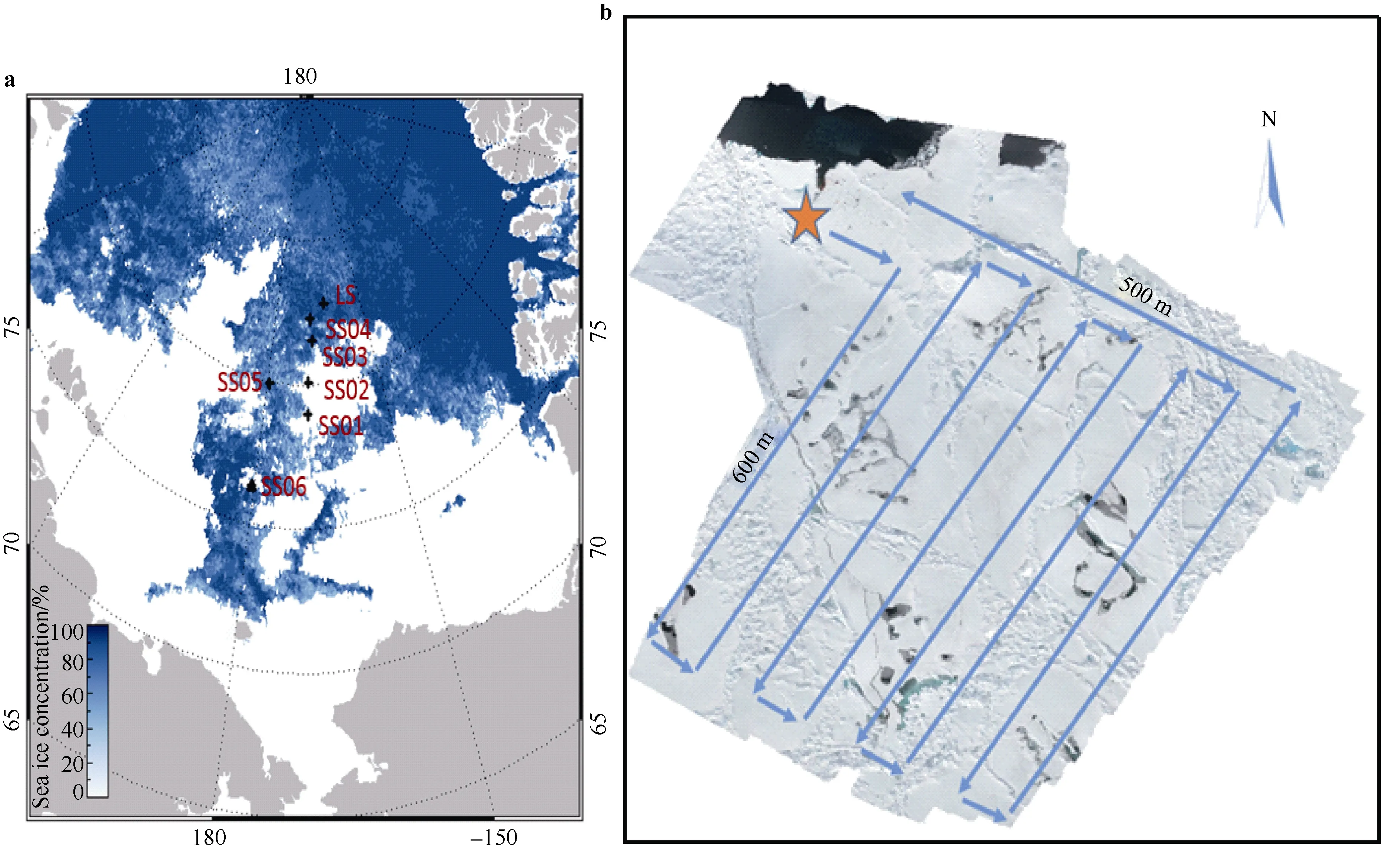
Figure 1 a, Location of the sea ice station SS06 deployed during the 7th Chinese National Arctic Research Expedition. The station is marked with a triangle. Color of the background of the image represents sea ice concentration derived from AMSR2 data on 20 August 2016. b, Flight trajectory of the UAV. Arrows indicate flight direction. Pentagram marks position of operation personnel. Background of the figure is the aerial photo mosaic.

2.2 Image acquisition

Observations were conducted from a DJI Phantom 4 micro UAV. Under low temperature conditions—between -5℃and 0℃—the UAV can stay in the air for more than 15 min with a single battery and with a maximum speed of 20 m·s-1.It collected data on ice floe surface characteristics over an area of 2.5 km around the station. Images were recorded by a camera mounted on the bottom of the UAV. The camera had a 1/2.3-inch SONY image sensor with 12.4 million pixels. To ensure image quality, flights were conducted as much as possible under sunny and low wind conditions.

On the basis of the distribution of sea ice in the study area, we decided to obtain images from a height of 100 m.This ensures coverage of a large sea ice area with sufficient detail so that the data can be used for 3D modeling of the ice surface. The UAV flew along bow-shaped lines with a side length of 500 m at an altitude of 100 m. Adjacent parallel lines were separated by a horizontal distance of 100 m with longitudinal and side overlaps of approximately 70%and 50%, respectively, obtaining an image over a sea ice area of 3.16×105m2(Figure 1).

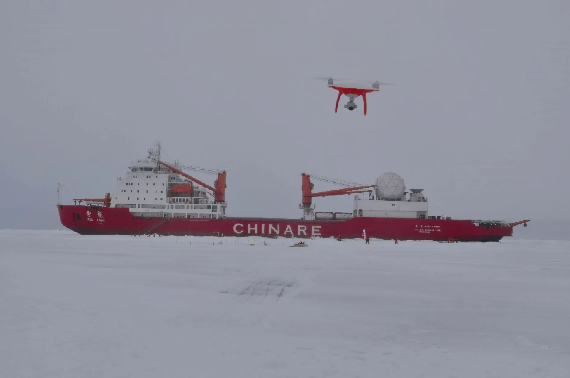
Figure 2 The DJI Phantom 4 UAV used for aerial photography and the R/V Xuelong icebreaker.

2.3 Image processing

In this section, we first describe a fog filtering process that we applied to our aerial images. Secondly, we present a melt pond discrimination method based on thresholds.Finally, we explain the procedure of the derivation of sea ice surface roughness from the DEM.

2.3.1 Fog filtering

Fog is a frequent phenomenon during the Arctic summer. It is difficult to discriminate between different sea ice surface types in aerial images obtained in foggy weather.

This problem also occurred in some of our images.Therefore, we used an improved dark channel prior based image defog algorithm to improve image quality (He et al.,2011). The dark channel prior defog method is based on the statistics of outdoor images. In fog-free outdoor images, the intensity of at least one color channel is very low or near zero in some pixels that lie outside the sky region. This channel is referred to as the dark channel. The dark channel intensity value is derived as follows:

where Jdarkrepresents the dark channel intensity value ; J, Jcrepresents the red (R), green (G), blue (B) intensity values of a small patch Ω(x) around the pixel x; Ω(x) is chosen as a function of the resolution and dimension of the image; it should be statistically significant and small enough to cover only one subject. Under fog-free conditions, the dark channel intensity value is nearly zero, and becomes higher when there is fog. Therefore the dark channel intensity value can be used to estimate fog thickness and calculate transmission, t(x), as follows:

where, ACis atmospheric background light intensity, which we assume to be at a constant value of 255. Once t(x) is calculated, a defogged image can be obtained using Equation (3):

where J(x) is the image before defogging, I(x) is the image after defogging. When applying the algorithm to our images,we found that the hypothesis that the dark channel intensity value is close to zero is not applicable to the bright, white surface of sea ice. In fact, the calculated dark channel intensity was too high, resulting in lower transmission values and errors in the defogged image. To solve this problem, a modified version of formula (2) was used when the dark channel intensity exceeded a prescribed threshold value of R:

The defogged image in Figure 3 shows a distinct sea–ice boundary, clear details of the sea ice surface, and sharp color differences indicating the presence of melt ponds.

2.3.2 Extraction of melt pond fraction

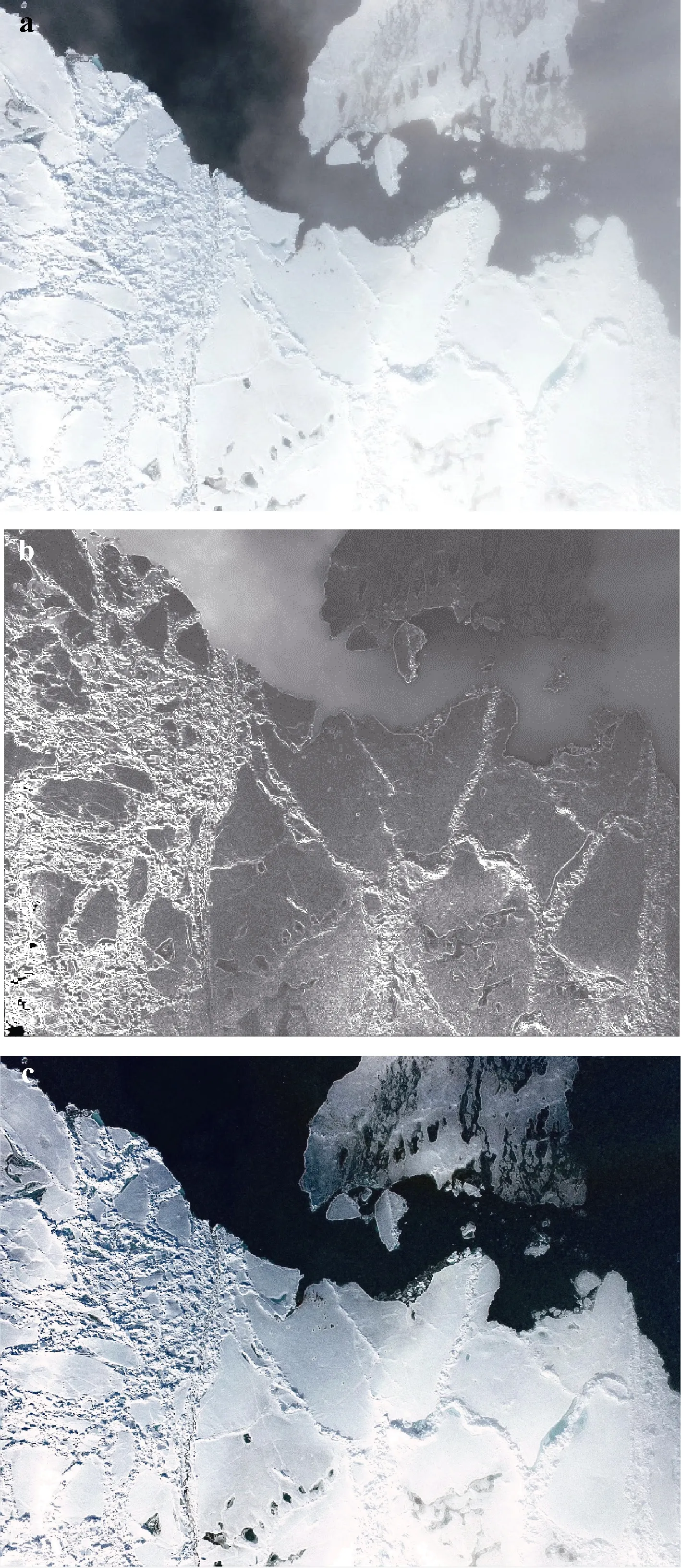
Figure 3 a, Image before fog filtering; b, Transmission map; c,Image after fog filtering.

To discriminate melt ponds in aerial images, the relationship between the gray value of the RGB channel and its spectral reflectance needs to be identified. Spectral reflectance was obtained in situ during the 7th Chinese National Arctic Research Expedition. Figure 4 shows the reflectance spectrum of some typical objects, including level ice, ridged ice, melt ponds and ice-covered melt ponds,the source of these data is explained in Section 2.4.Reflectance decreases as wavelength increases, peaking clearly at 600, 670, and 700 nm, and reaching minima at 630, 690, and 820 nm. The reflectance of frozen melt ponds is 15%–20% higher than that of liquid melt ponds. The reflectance of ridged ice is slightly higher than that of level snow-covered ice. The measured reflectance of melt ponds is higher than that reported previously (Perovich et al.,2003), which may be due to reflections coming from the snow surrounding the measurement instrument. Depressions in the snow have a lower reflectance than level ice because the reflected radiation is absorbed repeatedly by the wall of the depression. This indicates that, apart from melt ponds,ridged ice and depressions in the snow are also determining factors in the absorption of shortwave radiation of sea ice.Furthermore, these two factors also determine sea ice surface roughness. Calculations of sea ice surface roughness are introduced in Section 3.2.

Figure 4 Observed spectral albedo curves of different sea ice surface types. For each of the three rectangles: the width represents the spectral response range of the channels (R, G, B), it is defined as the wavelength interval where responsivity is higher than half of the highest responsivity of a certain channel, and the height represents normalized brightness intensity (R, G, B)of the melt ponds in domain D.

According to the above analysis, melt ponds, melt ponds that have melted through, and sea ice present different colors in an aerial image because of different reflectance in different wavelengths. As Figure 5 shows, the red channel intensities of melt ponds and melt ponds that have melted through are lower than that of sea ice. In melt ponds, the difference between the intensities of the red and blue channels and the difference between the intensities of the red and green channels are greater than that of sea ice and melt pond that have melted through. Thus, we define a parameter C as follows,

where Ri,j, Gi,j, Bi,jrepresent the intensities of the red, green,and blue channels, respectively. A higher value of C implies a greater difference between the red channel and the green and blue channels. We selected three training regions consisting of melt ponds, melt ponds that have melted through, and sea ice. The ranges of R and C in these regions are shown in Figure 5. Threshold values, R1 and C1, were identified manually from the histograms of R and C using Bayesian discrimination to allow melt ponds to be identified from aerial images (Figures 6e and 6f).

2.3.3 Sea ice surface roughness

The images were processed in Agisoft Photoscan. An orthogonal projection image with geographic information and a DEM with color texture were generated and georeferenced (Zhang et al., 2013) The DEM had a horizontal resolution of 1.94 m. Since the areal extent of human activity in our study area is small (as shown in Figure 6a) Ground Control Points (GCPs) were not used.Instead, we set the level ice surface as the reference plane,from which relative surface elevation can be calculated(Figure 7). Li et al. (2016) compared the three-dimensional coordinates generated by Photoscan with the actual coordinates of 24 control points, and found an overall elevation error of about 0.05 m, indicating a high precision in the DEMs generated by Photoscan.

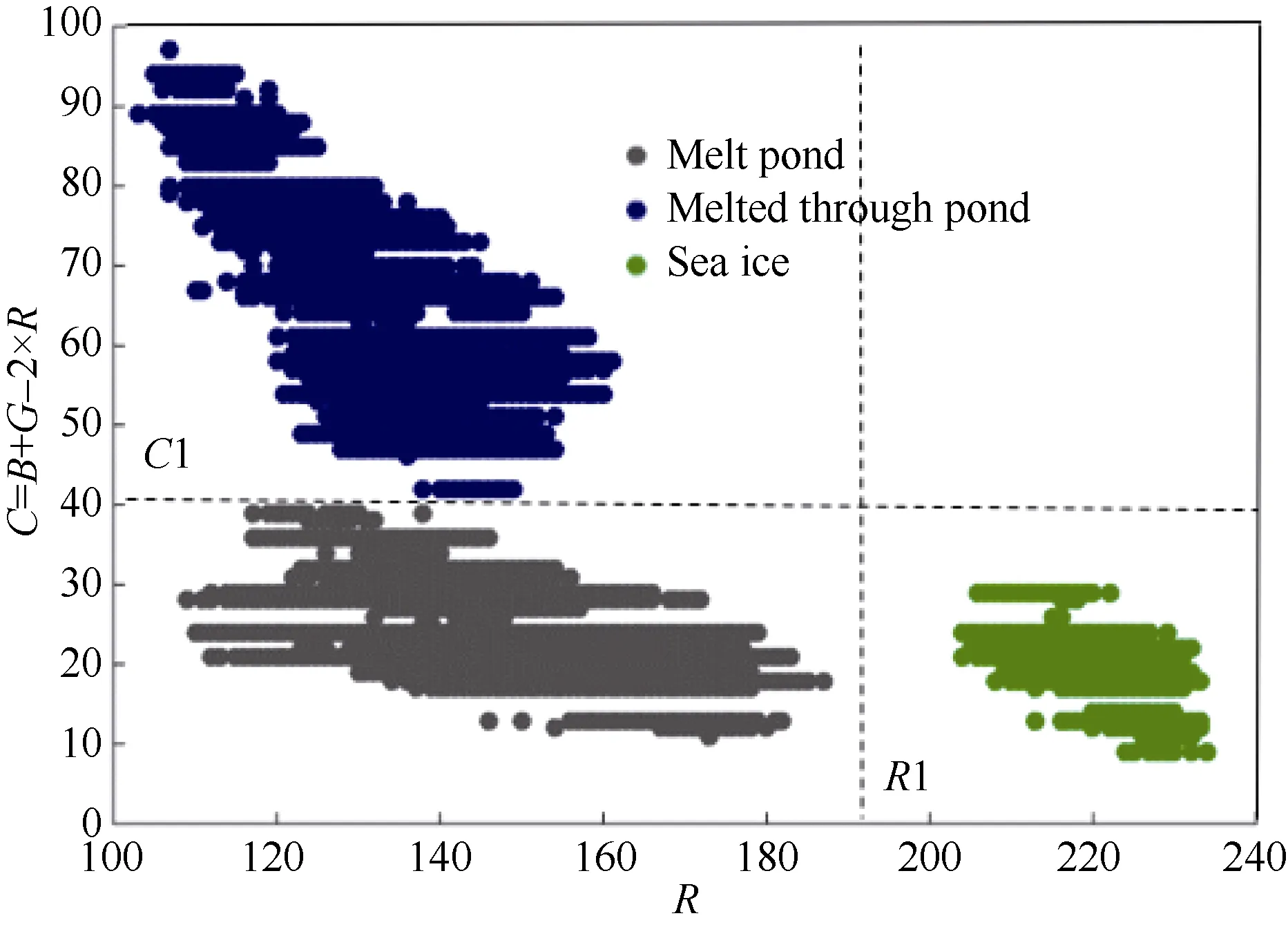
Figure 5 Melt pond discrimination. Blue, green and black dots represent melt ponds, melt ponds that have melted through, and sea ice, respectively. The x coordinate is the intensity value of the red channel of the aerial image. R1 and C1 are thresholds obtained from the histograms of R and C, respectively, using Bayesian discrimination.

Sea ice surface roughness strongly influences the location and depth of melt ponds. Together with wind speed,sea ice surface roughness is a key parameter for the determination of the latent and sensible heat coefficients at the air–ice interface (Andreas, 1987). These coefficients are,in turn, required for accurate simulations of the heat exchange at the snow and ice surface. Therefore, it is crucial to determine the values of sea ice surface roughness.

Sea ice surface roughness of a pixel is defined as the relative standard deviation of surface height within a window surrounding the pixel of interest. In a certain pixel numbered n, with a relative surface elevation of Hiand a mean relative surface elevation of Hin the chosen window,sea ice surface roughness R can be calculated using the following equation (Peterson et al., 2008):

Distribution of sea ice surface roughness was estimated using windows of 25 pixels arranged in a 5×5 grid (Figure 8b).

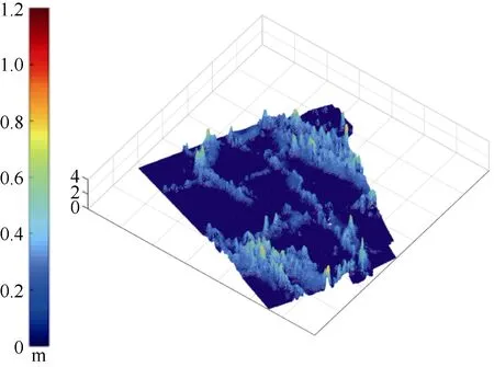
Figure 7 Digital elevation model of the study area.

2.4 Measurements of shortwave radiation

In this section, we describe the measurement of shortwave radiation and the calculation of reflectance for different sea ice surface types. Further, we provide support for the selection of the thresholds introduced in Section 2.3.2 with a discussion of RGB intensity of aerial images and reflectance.

Measurements of shortwave radiation from different sea ice surface types were conducted with the multi spectral radiometer MSR16R produced by Cropscan. The MSR16R makes vertical measurements, and has a spectral range from 460 to 1480 nm. It contains 32 detectors, which are arranged in pairs with one detector in each pair oriented upward and the other oriented downward. Each pair corresponds to a certain wavelength (450, 550, 577, 600,630, 650, 660, 670, 690, 720, 740, 770, 800, 900, 1000, and 1480 nm). The upward-facing detector receives downward solar radiation, while the downward-facing detector receives the radiation reflected by the ground. Thus, the reflectance of different ground objects is measured and radiation characteristics can then be analyzed.

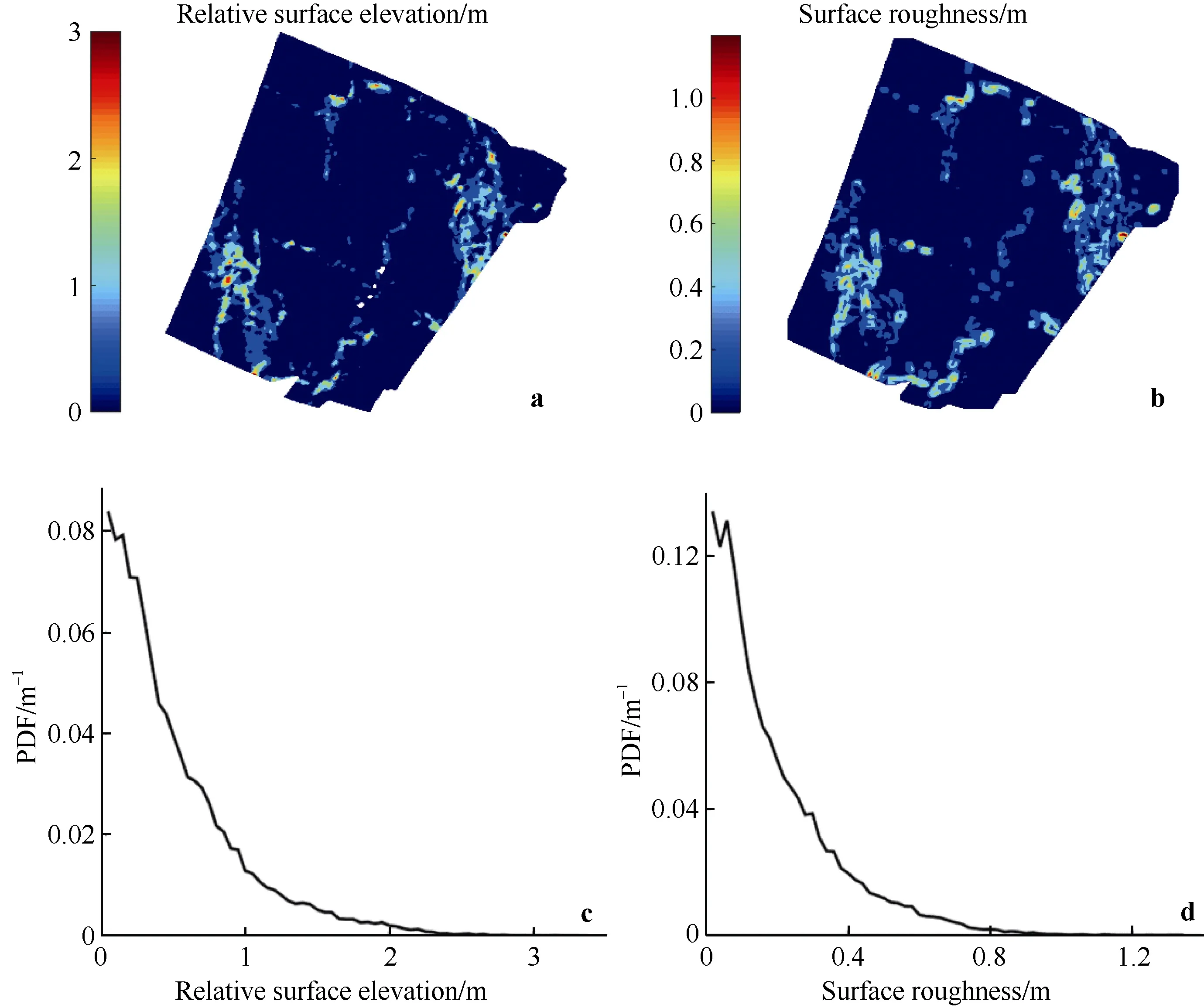
Figure 8 a, ice surface relative elevation derived from three-dimensional modeling based on aerial images; b, surface roughness of sea ice; c, Probability Density Function (PDF) of ice surface relative elevation; d, PDF of surface roughness of sea ice.

Aerial digital images are created when sunlight reflected by the sea ice surface penetrates the camera lens,passes through an infrared filter process, and stimulates the optical coupler, which then releases electrons creating electrical signals. Thus, pixel intensity can be used as a measure of light intensity of a certain wavelength. An algorithm for the discrimination of melt ponds can be developed on the basis of the relationship between reflectance and RGB channel intensities by normalizing the RGB channel intensities of the pixels identified as melt ponds (Domain D in Figure 6). The RGB channel intensities of aerial images were in good agreement with the measurements of the multi spectral radiometer despite a slight underestimation, which can be explained by two reasons. First, the aerial camera receives more atmospheric scattering than the MSR16R (compare the curves in Figure 4). Second, the camera’s charge coupled device is of limited quality, as on-site radiometric calibration processes require a charge coupled device with high spectral responsivity. In addition, the corresponding MSR16R spectral albedo curve was shorter than the spectral response range of the blue channel. So, we did not estimate the errors between the RGB channel intensities and radiometer measurements here.But, for further application, the method proposed will benefit from a camera with higher spectral response quality.

3 Results

After a fog filtering process, the 468 aerial images obtained at SS06 (red triangle in Figure 1) were spliced together using Photoscan, producing a final spliced image covering an area of 316000 m2and with a resolution of 2 cm (Left panel in Figure 6). Domain A in Figure 6 marks the location of the research ship. Domain D marks the region where shortwave radiation of melt ponds was measured. In domain D, a long, narrow, longitudinal lead (indicated with black arrows in Figure 6) extended northwards, and had a total length of approximately 621 m.

3.1 Melt pond fraction

Several melt ponds near the lead were at different status of melting. We retrieved melt pond fractions from two typical subareas (domains B and C in Figure 6) where melt ponds could be identified in the aerial images as light blue and green, respectively.

Melt ponds in domains B and C were identified using the method described in Section 2.3.2. Estimated melt pond fractions in domains B and C were 16.24% and 6.15%,respectively (Figures 6e and 6f). Total melt pond fraction in the study area was 1.63%. This fraction is considerably lower than other studies because our measurements were made in the last stage of the melt season and, since our objective was to validate the measurement technique, our field site was deliberately located in a region with low melt pond fraction for safety. Since different melt pond statuses present in varied colors, melt ponds are distinctive from each other in Figure 6. At station SS06, melt ponds in domain A and in the north of domain D were frozen.Cooling can cause the refreezing of melt ponds, altering their optical properties and the surface heat budget.

We used ERA-Interim data (Dee et al., 2011) to determine changes in thermodynamic parameters. As shown in Figure 9, around three days prior to the aerial observations, near surface temperature at a height of 2 m(T2m) decreased. Daily temperature minima clearly decreased (black dots in Figure 9), leading to a rapid decrease in ice surface temperature (Lt1). In-situ observations indicate that the melt ponds were mostly frozen on the surface. Freezing of melt ponds and sea water releases latent heat, increasing local cloud and water vapor,which can explain the large decrease in downward shortwave flux (Dsw) after 20 August 2016. Reductions in ice and air temperatures resulted in no apparent change in sensible heat flux (Fsin Figure 9). The exchange of energy between the atmosphere and the sea ice surface is given by

where Qisis the sea ice surface heat budget, Fsis the sensible heat flux, Flis the latent heat flux, Swis the net shortwave radiative flux, and Lwis the net longwave radiative flux.

Figure 9 shows that the sea ice surface heat budget (Qis)had been decreasing for a few days prior to the aerial observations. The ice surface was losing heat the night before the observations, indicating that the observed melt ponds were mostly frozen.

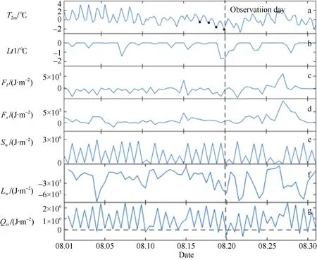
Figure 9 Thermodynamic parameters of the study area during 20 d prior to the day of aerial observations. T2m, air temperature at a height of 2 m; Lt1, surface ice temperature; Fl, ice surface latent heat flux; Fs, ice surface sensible heat flux; Sw, ice surface net shortwave radiative flux;Lw, ice surface net long wave radiative flux; Qis, sea ice surface heat budget; black dots in the T2m plot indicate a decrease in temperature.

Results indicate that pressure ridges covered up to 42%of the study area; they were scattered or arranged in strips(Figure 6). Mean relative surface elevation Hwas 0.22 m,while average sea ice surface roughness was 0.12 m.Relative surface elevation was highly correlated with surface roughness (Figures 8a and 8b), indicating that pressure ridges were the main factor influencing surface roughness. Relative surface roughness is mostly below 1 m with a maximum of 3 m, while surface roughness is almost below 0.4 m, and barely exceeding 0.8 m.

From the distributions of surface roughness (Figure 9b)and melt ponds (Figure 7), we can see that the surface roughness is high in regions where melt pond fraction and size are smaller. In contrast, low surface roughness is found in regions of level ice with broader melt ponds and where melt pond fraction is relatively high.

4 Summary and Discussion

This is the first study where Arctic melt pond and sea ice surface roughness were determined based on UAV aerial photography. We proposed a method to extract information on melt ponds and sea ice surface roughness from aerial images. The main conclusions are as follows:

(1) Sea ice images obtained by UAV in the Arctic should be defogged in the case of impacts of cloud and fog.We improved the transmission equation of the original dark channel prior defog algorithm, and developed a defog process that is applicable to aerial images of Arctic sea ice.

(2) We developed a method to identify and discriminate melt ponds from high-resolution aerial images.Melt pond fractions in the study area and two subareas were 1.63%, 16.24%, and 6.15%, respectively.

(3) We conducted a preliminary exploration of the retrieval of sea ice surface roughness utilizing a 3D modeling process, calculated mesoscale sea ice surface roughness (using Equation 6), and derived a regionally averaged surface roughness of 0.12 m. The distribution of melt ponds indicates that surface roughness is higher in regions where melt ponds are smaller in regions of level ice where broader melt ponds are found.

In general, during the summer melting season, melt pond fraction and sea ice surface roughness distribution are correlated. On level ice with low surface roughness, water in melt ponds can easily spread around the ice floe, forming larger melt ponds, which then deepen. Level ice is also usually thinner than ridged ice, and, therefore, can be melted more easily. In heavily deformed and ridged ice, it is difficult for water from melt ponds to spread. Therefore,melt ponds tend to develop downward, and have greater depths but smaller cross-sections.

Setting GCPs is needed for the 3D modeling process,but it is difficult to do so on Arctic sea ice because the areal extent of the ice station is small (as shown in Figure 6) compared with the UAV investigation area (the study area was located about 50 m from the ship, while the UAV ranged up to about 800 m from this site). Even if GCPS were set, they would be centralized in a small part of UAV investigation area and would be of little help for the generation of the DEM. Instead, we controlled the elevation by setting the level ice surface as the reference plane. The validity of this technique still needs further verification.

Compared with traditional methods of observations onboard ships and helicopters, the portability and high resolution of UAV observations provide a new and efficient tool for Arctic sea ice monitoring. Our method can be employed with fixed wing UAVs to enlarge the mapping area considerably. Time-lapse studies of melt ponds on sea ice surface are also possible. Moreover, this allows sea ice remote sensing products to be verified if aerial observation can be coordinated with the passage of satellites.

AcknowledgmentsThis work was funded by the National Natural Science Foundation of China (Grant no. 41276193), the Global Change Research Program of China (Grant no. 2015CB953901) and the National Key Research and Development Program of China (Grant no.2016YFC1402704). We are grateful to the 7th Chinese National Arctic Research Expedition team for providing access to the data. We also acknowledge Tina Tin and Yue Wu from the University of Southampton for providing English assistance in the drafting process.