Improved Teaching-Learning-Based Optimization Algorithm for Modeling NOX Emissions of a Boiler

Xia Li , Peifeng Niu , Jianping Liu and Qing Liu

Abstract: An improved teaching-learning-based optimization (I-TLBO) algorithm is proposed to adjust the parameters of extreme learning machine with parallel layer perception (PELM), and a well-generalized I-TLBO-PELM model is obtained to build the model of NOX emissions of a boiler.In the I-TLBO algorithm, there are four major highlights.Firstly, a quantum initialized population by using the qubits on Bloch sphere replaces a randomly initialized population.Secondly, two kinds of angles in Bloch sphere are generated by using cube chaos mapping.Thirdly, an adaptive control parameter is added into the teacher phase to speed up the convergent speed.And then, according to actual teaching-learning phenomenon of a classroom, students learn some knowledge not only by their teacher and classmates, but also by themselves.Therefore, a self-study strategy by using Gauss mutation is introduced after the learning phase to improve the exploration ability.Finally, we test the performance of the I-TLBO-PELM model.The experiment results show that the proposed model has better regression precision and generalization ability than eight other models.

Keywords: Bloch sphere, qubits, self-learning, improved teaching-learning-based optimization (I-TLBO) algorithm.

1 Introduction

Reducing NOXemissions of a boiler has been paid a significant attention recently in the economic development of power plants.In order to implement the reduction of NOXemissions, a precise model of NOXemissions firstly needs to be built.Due to the complex nonlinear relationship between the NOXemissions of the boiler and its influencing factors,it is difficult to build an accurate mathematical model by using mechanism modeling methods [Wang and Yan (2011)].Artificial neural networks (ANNs) based on datadriven modeling is an effective method in solving this problem [Zhou, Cen and Fan(2004); Ilamathi, Selladurai, Balamurugan et al.(2013)].However, the conventional neural network has the disadvantages of large amount of calculation, slow training speed,poor generalization ability and easy to fall into local minimum points.Extreme learning machine with parallel layer perception (PELM) [Tavares, Saldanha and Vieira (2015)] is a new type of neural network.In the PELM, the input weights and thresholds of hidden layer in the nonlinear part are randomly generated, and then the input weights and thresholds of hidden layer in the linear part are obtained by the generalized inverse of the matrix.The PELM has some good characteristics: Low model complexity, high calculation speed and good generalization ability.So, this network can overcome the shortcomings of back propagation (BP) neural network, such as large iterative calculation amount, slow training speed and poor generalization ability.In Tavares et al.[Tavares,Saldanha and Vieira (2015)], the PELM is applied to solve twelve different regression and six classification problems.The experiment results show that the PELM with high speed can achieve very good generalization performance.Furthermore, the PELM has the same regression ability as extreme learning machine (ELM) [Huang, Zhu and Siew(2006); Huang, Zhou, Ding et al.(2012)], but it only uses just a half of hidden neurons and has a much less complex hidden representation.So, the PELM is an efficient modeling tool, which can be used to solve various regression problems in real life.Therefore, in this study, the PELM is considered to build the model of NOXemissions of a boiler.Because the PELM randomly selects the input weights and thresholds of hidden layer in the nonlinear part, the regression precision and generalization ability may be affected.It is necessary to select the optimal input weights and thresholds in the PELM.Therefore, we need to find an efficient optimization algorithm to optimize the PELM.

Teaching-learning-based optimization (TLBO) algorithm is an intelligent optimization algorithm based on the teaching-learning in classroom [Rao, Savsani and Vakharia(2011); Rao, Savsani and Vakharia (2012)].This algorithm needs fewer parameters setting, but it can achieve higher calculation precision.The TLBO algorithm is simple in the concept, easy to understand, and fast in the calculation speed.Therefore, the TLBO algorithm has attracted many scholars’ attention and has been applied in many fields[Pawar and Rao (2013); Rao and Kalyankar (2013); Bhattacharyya and Babu (2016)].The TLBO algorithm has many advantages, but it also inevitably has some shortcomings.When it is used to solve some global optimization problems, the diversity of the population decreases with increasing number of iterations.It is very easy to fall into the local minimum and even stagnate.On the other hand, the convergent speed in the early stage is fast, but the convergent speed in the late stage gradually becomes slow.So the effectiveness of the TLBO algorithm is affected.

To overcome the shortcomings and improve the exploration ability and the exploitation performance of the TLBO, an improved TLBO (I-TLBO) algorithm is proposed in this study.In the I-TLBO algorithm, there are four major highlights.Firstly, quantum initialization by using the qubits on Bloch sphere replaces random initialization in original TLBO.This highlight can improve the quality of the initial population.Secondly,two kinds of angles in Bloch sphere are generated by using cube chaos mapping.The introduction of the cube chaos mapping can increase the diversity of the initial population.The search ability of ergodic to the solution space is improved.Thirdly, an adaptive control parameter is added into the teacher phase to speed up the convergent speed.And then, according to actual teaching-learning phenomenon of a classroom, students learn some knowledge not only by their teacher and classmates, but also by themselves.Therefore, a self-study strategy by using Gauss mutation is introduced after the learning phase to improve the exploration ability.The effectiveness of the I-TLBO algorithm is benchmarked on eight well-known testing functions.The performance of the I-TLBO algorithm is compared with particle swarm optimization (PSO) algorithm [Kennedy and Eberhart (1995)], grey wolf optimizer (GWO) algorithm [Mirjalili, Mirjalili and Lewis(2014)], TLBO algorithm, mTLBO algorithm [Satapathy and Naik (2013)], and TLBO with crossover (C-TLBO) algorithm [Ouyang and Kong (2014)].Wilcoxon signed rank test shows that the proposed I-TLBO algorithm is able to provide very good results compared to five other algorithms.So, the I-TLBO algorithm becomes a good selection to optimize the PELM, and a well-generalized I-TLBO-PELM model is obtained to predict NOXemissions of a boiler.

The rest of this study is arranged as follows.In Section 2, the PELM model and the TLBO algorithm are reviewed, respectively.In Section 3, the I-TLBO algorithm is proposed.In Section 4, the experimental study shows the validity of the I-TLBO algorithm.In Section 5, the I-TLBO-PELM model is proposed and is applied to model NOXemissions of the boiler.Finally, Section 6 concludes this study.

2 Basic concepts and related works

2.1 The model of the PELM

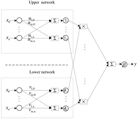
Figure 1: The structure of the PELM

The PELM was proposed by Tavares et al.[Tavares, Saldanha and Vieira (2015)].The structure of the PELM is described in Fig.1.Suppose a data set withNarbitrary distinct samplesthe PELM has m hidden layer nodes.U is the matrix of the weights and the thresholds of hidden layer in the upper network.Vis the matrix of the input weights and thresholds of hidden layer in the lower network.are activation functions.Then, the PELM is mathematically modeled as

wherea jlandbjlare

ujiandvjiare the elements ofUandV;xilis theith input of thelth sample andylis the output of thelth sample.In the PELM, the input-output mapping is made by applying the product of functions [Tavares, Saldanha and Vieira (2015)].

As a particular case of Eq.(1), whenβ(·)andγ(·)are linear functions, the network outputylis computed as

Substituting Eqs.(2) and (3) into Eq.(4), we can obtain Eq.(5)

In Eq.(5),vjiof the nonlinear part is randomly selected in [-1,1], and thenujiof the linear part is obtained by the least square method.

2.2 An introduction of the TLBO algorithm

The TLBO algorithm simulates the influence of a teacher on learners in a class teaching to obtain the global optimal solution.Compared with other nature-inspired algorithms,The TLBO algorithm has the advantages of the simple principle, the few parameters and the high precision.In the TLBO, the learners are considered as the populationX.The teacher is considered as the most knowledgeable person in a class and shares the knowledge to the students to improve the marks of class.The learning result of a learner is analogous to the fitnessis the size of the population.There are two parts in the TLBO: The teacher phase and the learner phase.The teacher phase means that students learn the knowledge from the teacher.The learner phase means that students learn the knowledge from the classmates by communicating with each other.

2.2.1 The teacher phase

In this stage, the teacher teaches individual knowledge to their students to improve the average level of the students in whole class.The students learn the knowledge from teachers to narrow the gap between the teachers and the students.LetMdenote scores before and after study, respectively.The average level of the students in the whole class isThe teacher tries to raise the level of students toby differential teaching.Then the whole teaching process can be expressed as

AcceptXnew,i, if it gives a better function value.

2.2.2 The learner phaseAfter the teacher has finished teaching, the knowledge levels of the students have been improved.However, the individual level of every student is different from others, so the students can still learn new knowledge from other superior individuals.At the stage of mutual learning among students, the studentXirandomly selects another studentXj(ij) by contrast learning.The process of learning among the classmates is

AcceptXnew,i, if it gives a better function value.The algorithm will continue its iterations until reaching the maximum number of iterations.

3 An improved TLBO （I-TLBO）algorithm

The parameter setting of the TLBO algorithm is fewer and the calculation precision is higher.However, the TLBO is also easy to fall into a local minimum, and it can not find the optimal solutions.Therefore, an improved TLBO algorithm called I-TLBO algorithm is proposed.In the I-TLBO algorithm, there are four major highlights, which are expressed in detail as follows.

3.1 Quantum initialized population by using the qubits on Bloch sphere

In general, population-based optimization techniques start the optimization process with a set of random solutions, but they need sufficient individuals and iterations to find the optimal solution [Mirjalili (2016)].Vedat et al.[VedatandAyşe (2008)] pointed out that initial population of high quality could reduce the number of search to reach the optimum design in the solution space.The initial solutions were coded by using Bloch spherical coordinates, which expanded the quantity of the global optimal solution and improved the probability to obtain the global optimal solution [Huo, Liu, Wang et al.(2017)].Because the original TLBO algorithm uses a randomly initialized population, it is difficult to guarantee that the population has good quality solutions.For overcoming the defect, the population is generated by using qubits based on Bloch spherical coordinate.The detailed scheme is described in this part.

In quantum computing, a qubit represents the smallest unit of the information, whose state can be expressed by Eq.(9)

where the anglesϕandθcan determine the point on the Bloch sphere [Li (2014)].Representation of the qubit on Bloch sphere is shown in Fig.2.

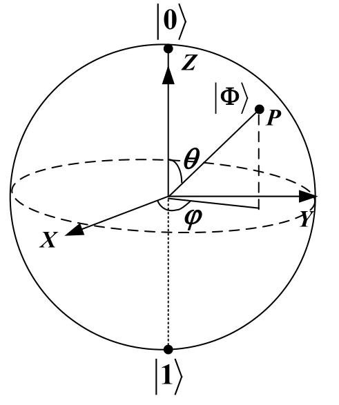
Figure 2: Representation of the qubit on Bloch sphere

According to Fig.2, a qubit corresponds to a point on the Bloch sphere.Therefore, a qubit〉can be presented by using the Bloch spherical coordinate in Eq.(10).

wheredis the dimension of the optimization space,Each initial solutionPicorresponds to three locations on Bloch sphere, which is shown in Eq.(14).They are on X axis, Y axis and Z axis, respectively.

According to the relationship between the qubits and the coordinates of the points on Bloch sphere, the global optimal solutionP∗is possibly obtained on the three circles [Li(2014)], which is shown in Fig.3.

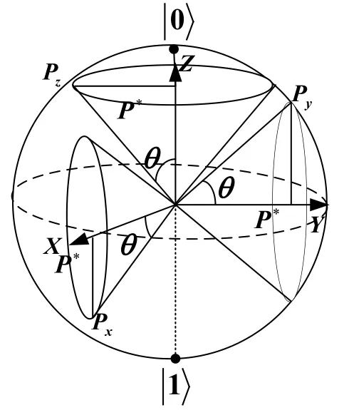
Figure 3: A pointP∗corresponds to three circles on Bloch sphere

Letjth dimension ofPibeon Bloch sphere.The range of thejth dimensionin the original solution space.So, the transformation formula from Bloch sphere to the original solution space is shown in Eq.(15)

Then selectMindividuals with the best fitness values as the initial population among all 3Mcandidate solutions.Because the initial solutions of high quality are possibly obtained from three coordinate axes, the number of initial solutions of high quality is extended.Thereby, the introduction of quantum mechanism increases the convergent probability.This highlight makes the I-TLBO algorithm more easily find the global optimal solution.

3.2 The angles ϕij and θij are generated by using cube chaos mapping

The anglesϕijandθijin Eqs.(12-13) are randomly generated by using the uniform distribution.Therefore, a random initialization reduces the search efficiency of the algorithm to some extent.Chaos is a kind of universal nonlinear dynamic phenomenon,and the chaotic motion can traverse all states according to its own law within a certain range.This advantage can be used as an effective method to avoid falling into a local minimum.Because of the ergodicity of the chaos, the initialized population by using chaos is diverse enough to potentially reach every mode in the multimodal functions[Gandomi and Yang (2014)].Jothiprakash et al.[Jothiprakash and Arunkumar (2013)]generated the initial population for Genetic algorithm (GA) and Differential Evolution(DE) algorithm by chaos theory and applied it to a water resource system problem.They showed that GA and DE with initial chaotic populations outperformed those of the standard GA and DE algorithm.Furthermore, the combination of chaos and metaheuristic optimization algorithms has a faster iterative search speed than the uniform distribution [Coelho and Mariani (2008)].All these studies show the potential of chaos theory for improving the performance of the optimization algorithms.

The literature [Zhou, Liu and Zhao (2012)] proved that cube chaos mapping based on time series has good homogeneity.Therefore, we generateϕijandθijby using the cube chaos mapping, which is shown in Eq.(16).

The detailed implement process of the cube chaos mapping in the I-TLBO algorithm are given as follows:

Randomly generate twod-dimensional vectorsandEach component of these two vectors is between 0 and 1.

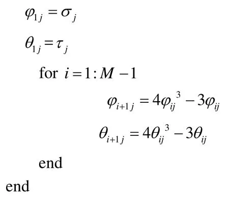
Because the introduction of cube chaos mapping can increase the diversity of the population, it expands the ergodic ability to search solution space.Therefore, the highlight improves the quality of the initial population once again and enhances the global exploration ability of the TLBO algorithm.

3.3 An Adaptive control parameter in the teacher phase

In order to balance the local exploitation ability and the global exploration ability of TLBO algorithm, an adaptive control parameter, as shown in Eq.(17), is proposed in the teacher phase.

Eq.(6) is changed into Eq.(18) below in the teacher phase.

In Eq.(17),andare the maximum value and the minimum value of the control parameter, respectively;tis the current iteration number, andGis the maximum iteration number.A larger value ofwfacilitates the global exploration, while a smaller value ofwfacilitates the local exploitation.Selecting suitable value ofwcan provide a balance between the global exploration and the local exploitation.Therefore, in Eq.(17),the control parameterwnonlinearly decreases with increasing of the number of iterations.This highlight makes the algorithm advantageous to the global exploration in the early stage and the local exploitation in the late stage of the iteration.

3.4 A self-learning process by using Gauss mutation after the learner phase

In the TLBO algorithm, the students only improve their marks by learning from their teacher and classmates.In fact, the students not only rely on others to learn some knowledge, but also they often make unremitting efforts by themselves to improve their marks in actual learning.So inspired by the idea of self-learning to gain some knowledge,we add the self-learning process after the student phase.We implement the self-learning process by using Gauss mutation.This highlight is used to improve the exploration ability against the premature convergence.The self-learning process is illustrated as follows.

wherehis the step size;Xiis the current best solution in learner phase;abs(Xi)denotes the absolute value of the elements ofXi, andrandnis a Gauss random number.AcceptXnew,i, if it gives a better function value.

The flow chart of the I-TLBO algorithm is shown in Fig.4.By adding above four improvements, we enhance the exploration ability and exploitation ability of the TLBO algorithm.Therefore, the optimization capability of the I-TLBO algorithm is better than the TLBO algorithm.This analysis is consistent with the following simulation results.

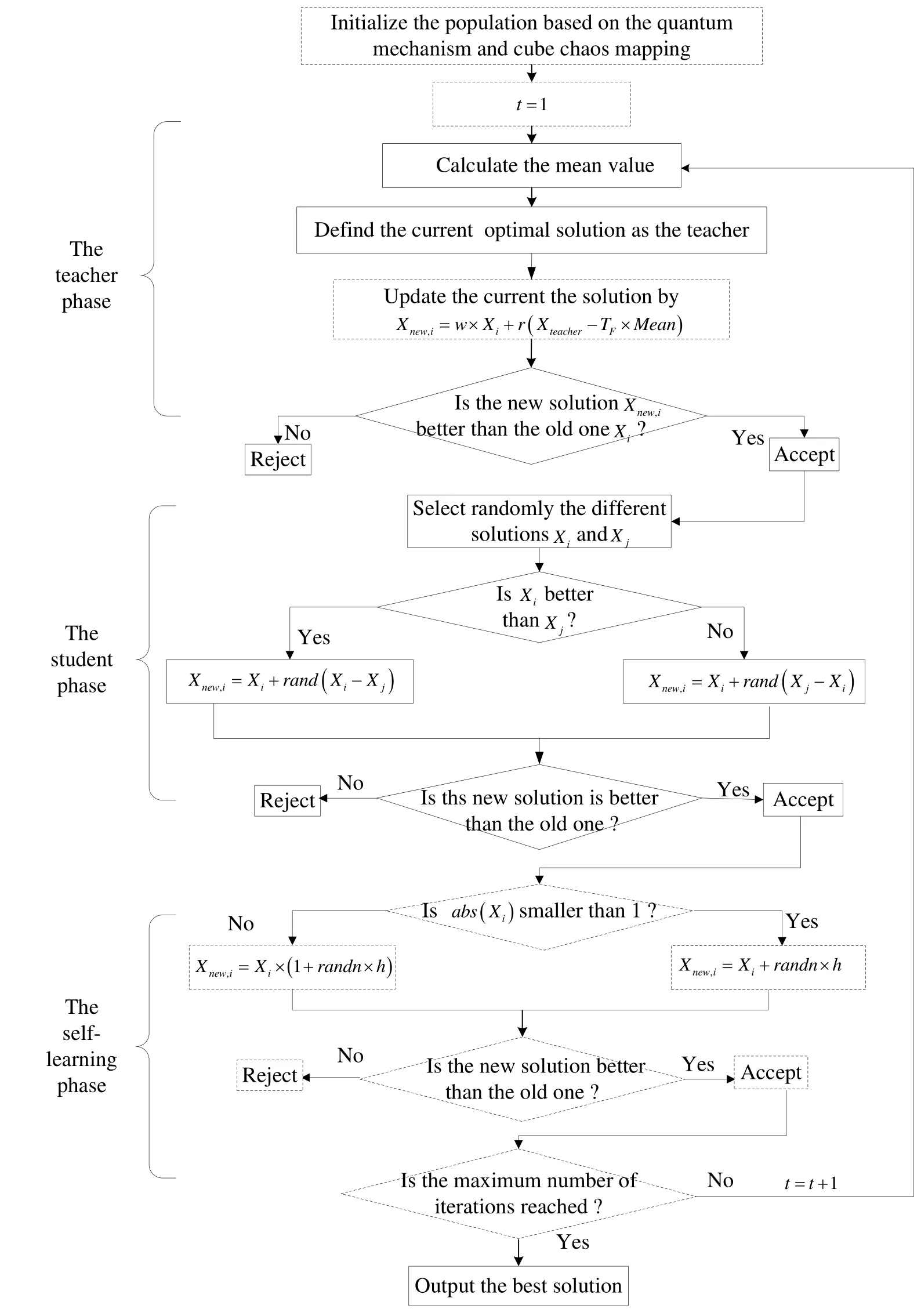
Figure 4: The flow chart of the I-TLBO algorithm

4 The simulation experiments on the benchmark functions

The optimization performance of the I-TLBO algorithm on a test of benchmark functions is compared with the PSO, GWO, TLBO, C-TLBO, and mTLBO.The performance of the proposed algorithm is verified on eight classic benchmark functions.

4.1 The classical benchmark functions

These benchmark functions [Rashedi, Nezamabadi-Pour and Saryazdi (2009); Mirjalili,Mirjalili and Lewis (2014)] are the classical functions utilized by many researchers,which are shown in Tab.1.F1-F4is unimodal benchmark functions, which are used to verify exploitation ability of fast finding the optimal solutions.The convergent speeds of unimodal benchmark functions are more interesting than the final results of optimization.F5-F8are used to verify the exploration ability of finding the global optimal solutions.For the multimodal functions, the computation results are much more important.They reflect an algorithm’s abilities of escaping from poor local optima and finding a good nearglobal optimum [Xin, Liu and Lin (2002)].

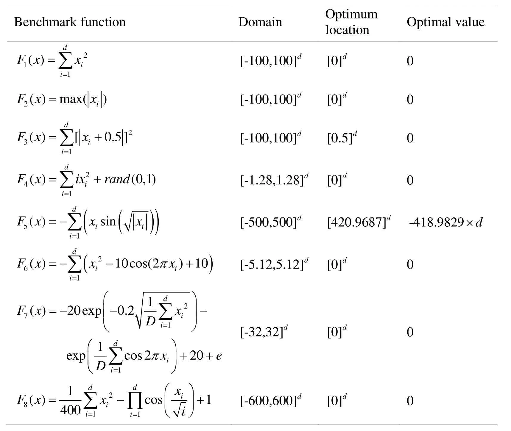
Table1: The classical benchmark functions

4.2 The experiment study and results analysis

All the programs are run under MATLAB 2009a environment in Windows 7, 2.2 GHZ CPU.Every experiment is repeated 10 times.The best value, the mean and the standard deviation (S.D.) of the best function values have been recorded for six algorithms.In order to fairly compare the computation results, six algorithms use the same population sizeM=30and the maximum number of generationsIn the PSO,In the C-TLBO, the crossover factor (CR) is set as 0.95, which is the same as [Ouyang and Kong (2014)].In the I-TLBO, after a lot of experiments, the values ofh,wstartandwendare all set as 0.03, 0.08 and 0.01 respectively.The experiment results are given in Tabs.2-3 and Fig.5.The best results are displayed in the bold face.

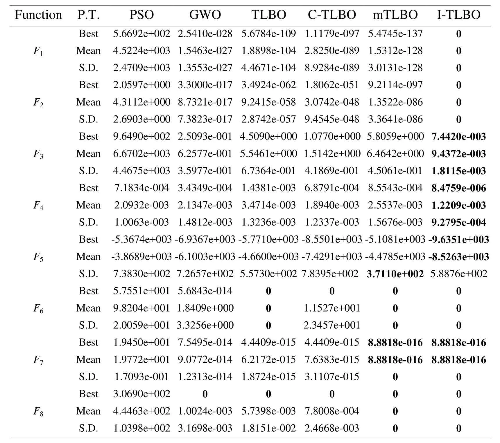
Table 2: Computational results of six algorithms when d=30

As seen from Tab.2, whend=30, the I-TLBO algorithm presents the best value and the lowest mean in all eight functions and the lowest S.D.in seven functions exceptF5.The mTLBO algorithm shows the lowest S.D.onF5, but the best value and the mean are much worse than the I-TLBO algorithm.The mTLBO algorithm also presents the best value, the lowest mean and S.D.onF6-F8.The TLBO algorithm also presents the best value, the lowest mean and S.D.onF6.However, from Fig.5, we can see that the convergent speed of the I-TLBO algorithm is much faster than the mTLBO and the TLBO onF6-F8.

As seen from Tab.3, whend=50, the I-TLBO algorithm presents the best value and the lowest mean in all eight functions and the lowest S.D.in seven functions exceptF5.The mTLBO algorithm shows the lowest S.D.onF5, but the best value and the mean are much worse than the I-TLBO algorithm.The TLBO algorithm also presents the best value, the lowest mean and S.D.onF6andF8.The mTLBO algorithm also presents the best value, the lowest mean and S.D.onF6-F8.However, from Fig.5, we can see that the convergent speed of the I-TLBO algorithm is much faster than the TLBO and the mTLBO onF6-F8..

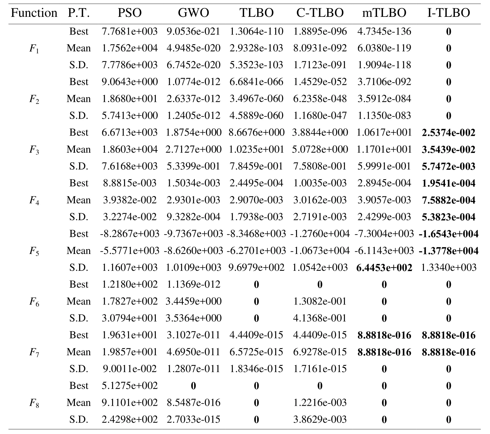
Table 3: Computational results of six algorithms when d=50

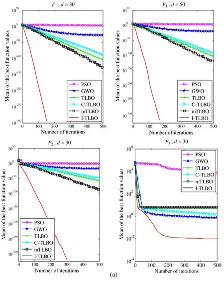
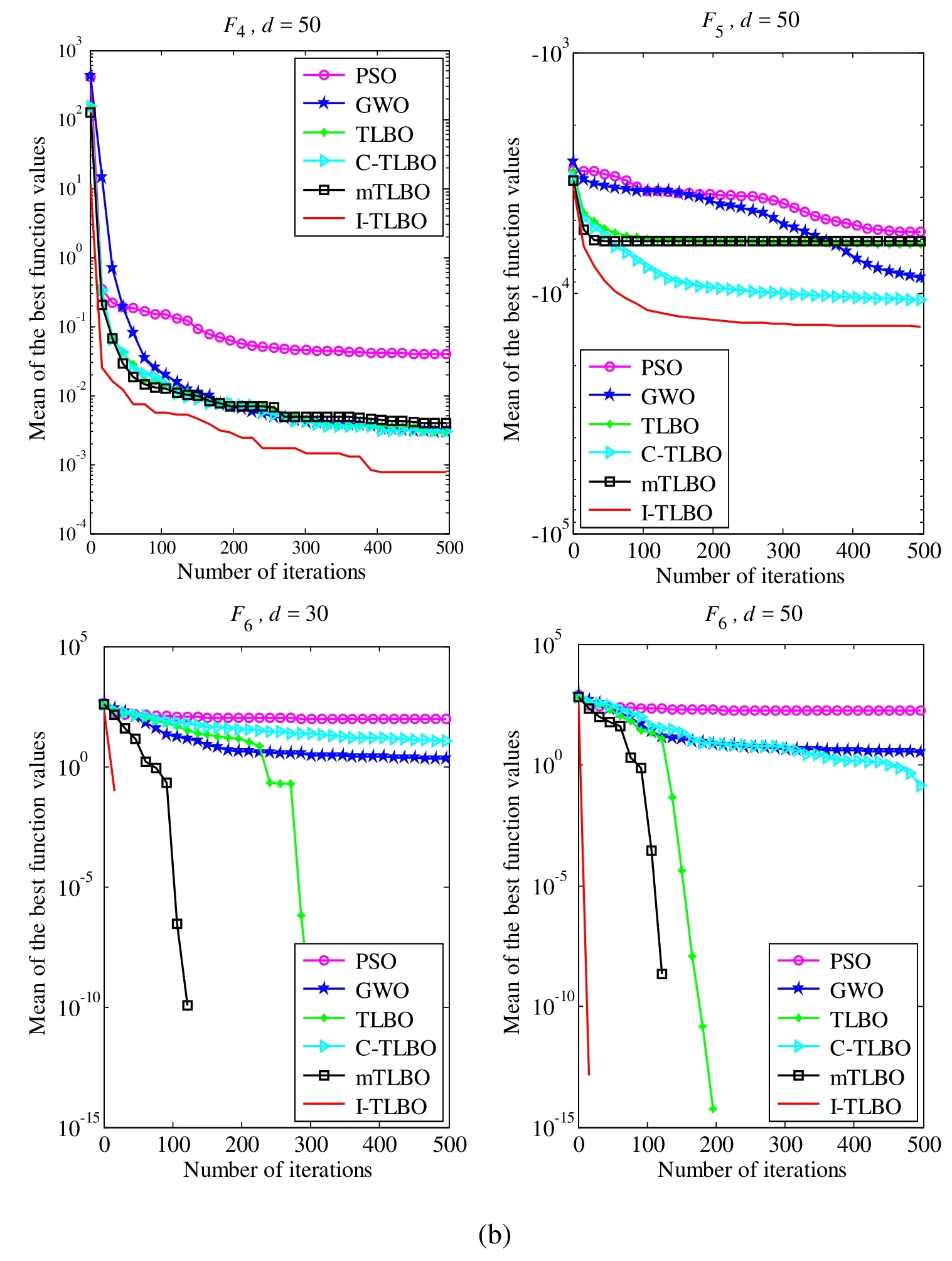
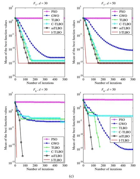
Figure 5: Performance comparison of six algorithms on the benchmark functions

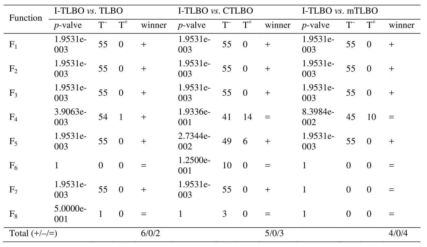
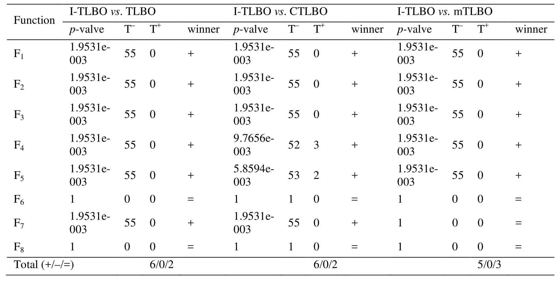
Wilcoxon signed rank test is devoted to detecting possible differences between the ITLBO and five other optimization algorithms.The “+”, “=” and “-” denote that the performance of the I-TLBO algorithm is better than, similar to and worse than that of the corresponding algorithm, respectively.The significance level is set as 0.05.As seen from the results of statistical tests in Tabs.4-5, the I-TLBO algorithm is significantly better than five other algorithms on the unimodal functions and the multimodal functions.From the above analysis of the experimental results, it has been found that whether on unimodal or multimodal functions, whetherthe I-TLBO algorithm is superior to five other optimization algorithms.Therefore, the I-TLBO algorithm is an excellent optimization algorithm, and can be applied to optimize the PELM for modeling NOXemissions of a boiler.

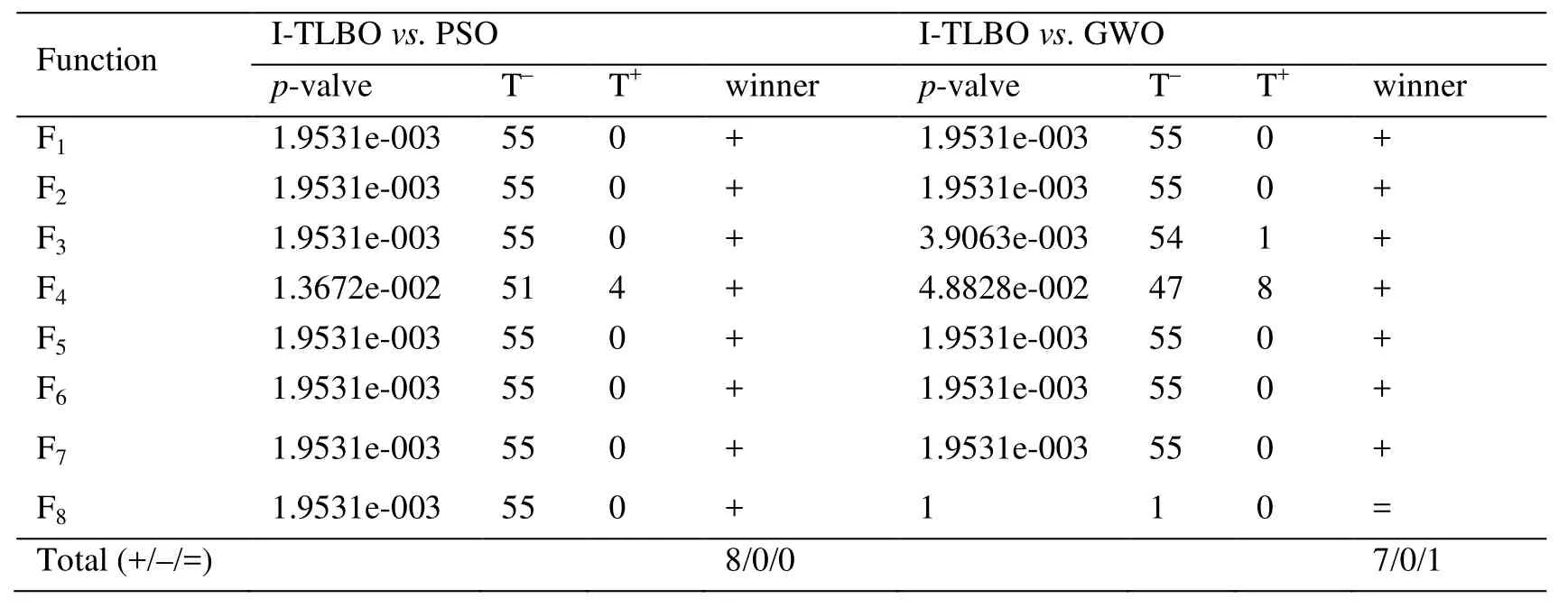
Table 4: The statistical comparison of the six algorithms by Wilcoxon signed-rank test for d=30

(Continued)

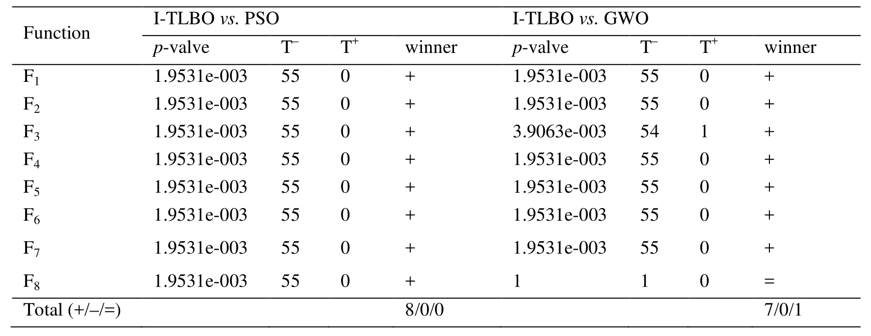
Table 5: The statistical comparison of the six algorithms by Wilcoxon signed-rank test for d=50

(Continued)

5 Model the NOX emissions based on the I-TLBO algorithm and PELM

With the development of coal-fired power stations, combustion technology of low NOXemission has become an important research direction of boiler engineering.In order to reduce pollutant emissions, NOXemissions model firstly needs to be built.The NOXemissions model depends on various operating parameters, such as air velocity, coal feeder rate, oxygen content in the flue gas, exhaust gas temperature.However, due to the complexity, uncertainty, strong coupling, and the nonlinearity of the combustion process,it is difficult to use the theory of thermodynamics to model the NOXemissions.The PELM is a new intelligent modeling tool based on the history combustion data of a boiler.In the PELM, the input weights and thresholds of hidden layers in the nonlinear part are randomly generated.To improve the generalization performance of the PELM, it is necessary to select the optimal input weights and hidden thresholds.Therefore, we select proposed I-TLBO algorithm to optimize the PELM and build I-TLBO-PELM model of NOXemissions.

There are rooms and halls in it, but we do not enter them, weremain in the kitchen, where it is warm and light, clean and tidy; thecopper utensils13 are shining, the table as if polished with beeswax;the sink looks like a freshly scoured14 meatboard

5.1 An introduction of the data

There are 240 data samples collected from a boiler, which are sampled once every 30 s and listed in Tab.6.100% load, 75% load and 50% load have 80 samples, respectively.In this study, the total 240 cases are divided into two parts: 192 cases (64 for 100% load,64 for 75% load, and 64 for 50% load) as the training data, and the remaining 48 cases as the testing data.The NOXemission is as the output variable, and 20 operational conditions closely related to the output variable are as the input variables of the I-TLBOPELM model.The 20 operational conditions are given as follows.

The boiler load (%);

The fluid bed temperature (FBT,oC);

The coal feeder rate (CFR, th-1), including A level, B level, C level and D level;

The primary air velocity (PAV, kNm3h-1), including left level and right level;

The primary air temperature (PAT,oC), including left level and right level;

The secondary air velocity (SAV, kNm3h-1), including left and inside level, left and outside level, right and inside level, right and inside level.

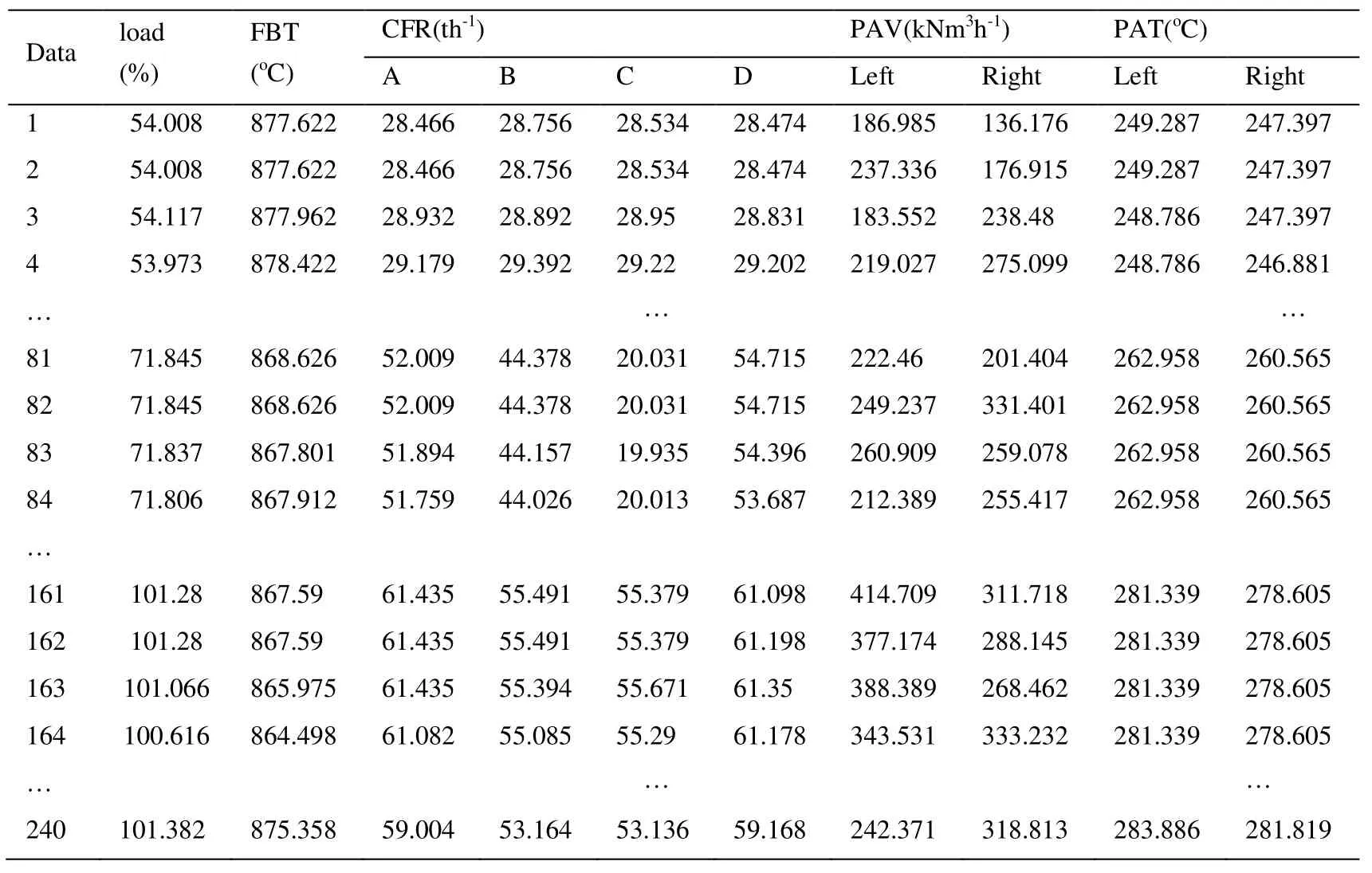
Table 6: The boiler operating conditions

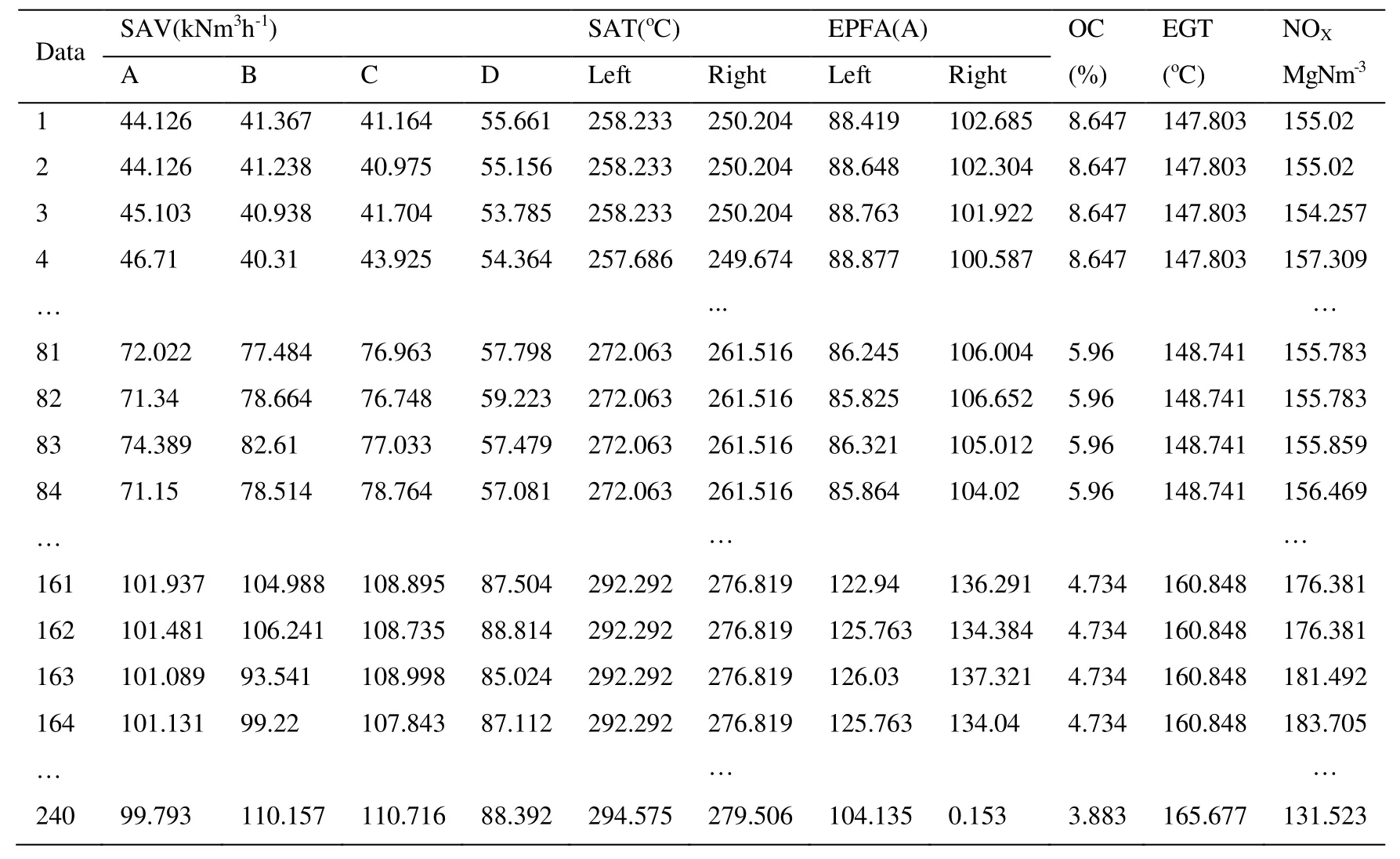
Continued

The electricity of powder feeding machine (EPFM, A), including A level and B level;

The oxygen content in the flue gas (OC, %);

The exhaust gas temperature (EGT,oC).

5.2 Model the NOX emissions by using the I-TLBO-PELM

According to Caminhas et al.[Caminhas, Vieira and Vasconcelos (2003); Tavares,Saldanha and Vieira (2015)], although the PELM requires much smaller number of hidden neurons than other ANNs, it can still obtain the good generalization capability and approximation performance.After a lot of experiments, 3 neural nodes are set in the PELM.The activation function is sigmoid functionThe maximum iteration number of six optimization algorithms is set as 100.All other parameter settings are the same as those of the Fourth part.The optimization object function is the root mean square error (RMSE) on the training data as follows:

whereNis the number of the training data and

The detailed modeling process by using the I-TLBO-PELM is summarized in the following steps.

Step 1: Set the control parameters of the I-TLBO algorithm, such as the size of the populationM, the maximum number of iterationsG, the values ofwstartandwend;

Step 2: Initialize the population based on the quantum mechanism and cube chaos mapping.The population is composed ofMindividuals;

Step 3: Evaluating the fitnessf(η)of each individualηby using Eq.(20);

Step 4: Optimizeηbased on the teacher phase, student phase and self-learning phase;

Step 5: If the maximum number of iterationsMis reached, the I-TLBO algorithm is stopped; otherwise, renew the population of the I-TLBO algorithm and the iteration is repeated from Step 4;

Step 6: The optimalηis obtained, and thenηis substituted in Eq.(5).We can obtain the optimal PELM model and then the model is applied to predict the NOXemissions on the testing data.

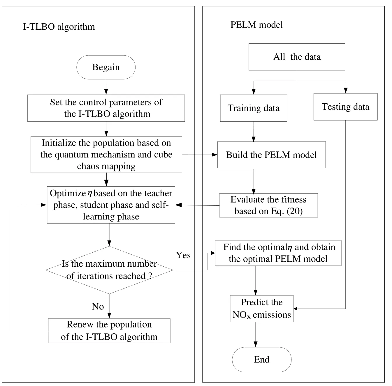
Figure 6: The modeling process of the I-TLBO-PELM

For a more vivid observation, the realization flowchart of the proposed I-TLBO-PELM is shown in Fig.6.

In addition, RMSE, mean absolute error (MAE) and mean absolute percentage error(MAPE) are used to evaluate the performance of the I-TLBO-PELM model.We compare with the PELM model, the PSO-PELM model, the GWO-PELM model, the TLBOPELM model, the mTLBO-PELM model and the C-TLBO-PELM model.Additionally,in order to test the superiority of the I-TLBO-PELM model, we also compare with BP neural network and linear regression (LR).Although there are many variants of BP algorithm, a faster BP algorithm called Levenberg-Marquardt algorithm provided by MATLAB package is used in our simulations.The comparison results of the training data and the testing data are given in Tabs.7-8 and Figs.7-8.

5.3 The experiment results and analysis

As shown in Tab.7, for the I-TLBO-PELM model, the RMSE is 4.1763, the MAE is 3.1867, and the MAPE is 0.0228.Three performance indexes of the I-TLBO-PELM are smaller than those of eight other models.Therefore, the approximate ability of the ITLBO-PELM is the best in nine models.

For the testing data, for the I-TLBO-PELM model in Tab.7, we can see that the RMSE is 4.9068, the MAE is 3.9174, and the MAPE is 0.0276.Every performance index is also the smallest in nine models.So, the I-TLBO-PELM model has the best generalization and predicted performance in nine models.

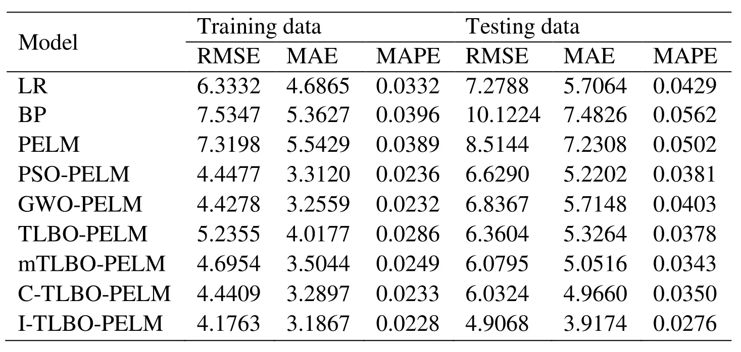
Table 7: Performance comparison for the NOX emissions

Fig.7 shows predicted NOXemissions of nine models on the testing data.As seen from it,the predicted values of the I-TLBO-PELM model are very closer to the actual values than eight other models.The relative errors of the testing data are given in Fig.8.The range of the error fluctuation of the I-TLBO-PELM model is about in [-0.06, 0.06].The ranges of eight other models are larger than the I-TLBO-PELM.Therefore, the I-TLBO-PELM is more accurate for modeling the NOXemissions of the boiler than eight other models.

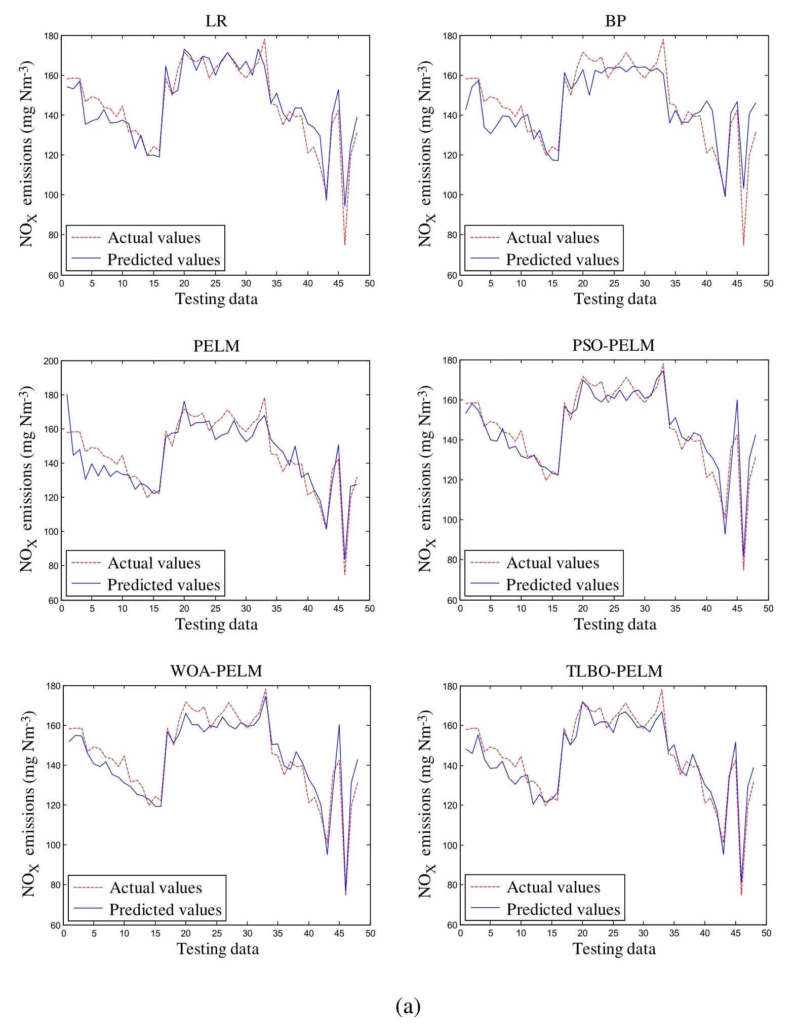
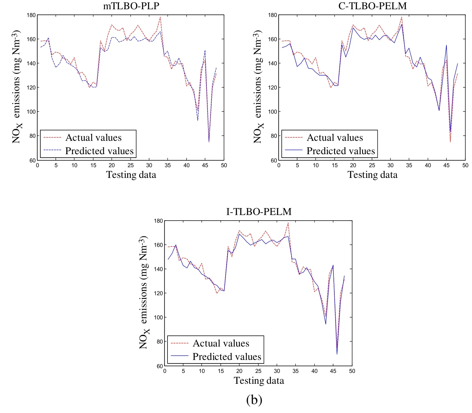
Figure 7: Predicted NOX emissions of nine models on testing data

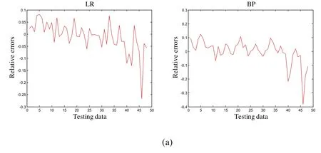
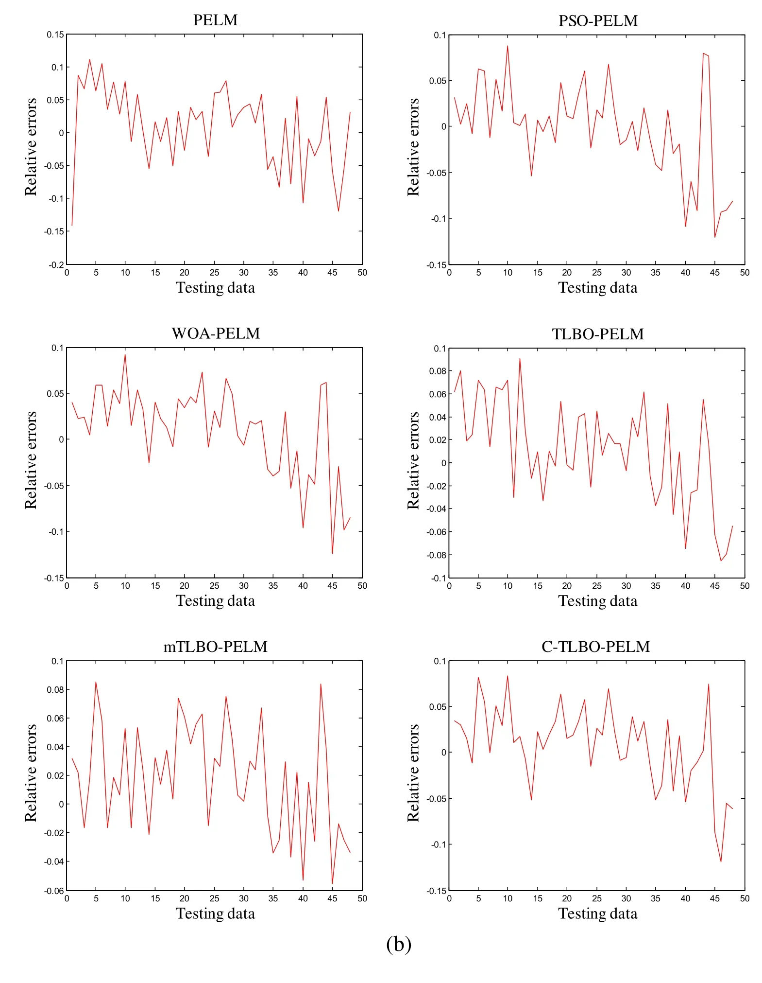
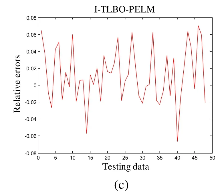
Figure 8: Relative errors of nine models on testing data

Moreover, in order to further verify that I-TLBO-PELM is a better modeling tool under different experiments conditions, 5% white noise is added into the target attribute of the data.For noise-added data, the parameters of employed methods are the same as the data without noise in order to well compare the robustness of all models to perturbations [Li and Niu (2013)].The comparison results of the training data and the testing data are shown in Tab.8.

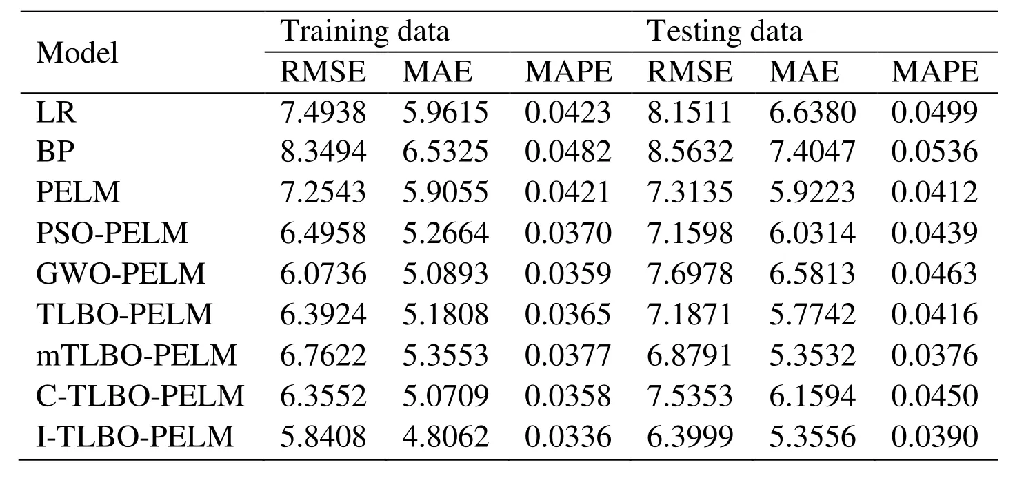
Table 8: Performance comparison for the NOX emissions under the condition of 5%noise

As seen from Tab.8, whether on the training data or on the testing data, every performance index of the I-TLBO-PELM model is also the smallest in all nine models.It shows that the I-TLBO-PELM model owns a good robustness and can competently reduce the adverse effects which are caused by the perturbation.

In summarize, the proposed I-TLBO-PELM model is relative accurate.This model has very good approximate ability, generalization performance and robustness.So, the ITLBO-PELM can provide an effective method to predict the NOXemissions of the boiler working.

6 Conclusions

In order to improve the exploration ability and exploitation performance of the TLBO algorithm, an I-TLBO algorithm is proposed.In the I-TLBO, there are four improvements.Firstly, the quantum initialized population based on qubits replaces the randomly initialized population.Secondly, two kinds of angles in Bloch sphere are generated by using the cube chaos mapping.Thirdly, an adaptive control parameter is added into the teacher phase.And then, a self-learning process by using Gauss mutation is proposed after the learner phase.The optimization performance of the I-TLBO algorithm is verified on eight classical optimization functions.The experimental results show that the I-TLBO algorithm not only can jump out of the local optimal solution so as to achieve the global optimal solution, but also the convergent speed is the fastest in the six algorithms.Finally, a hybrid I-TLBO-PELM model is built to predict NOXemissions of a boiler.Compared with eight other models, the I-TLBO-PELM model has good regression precision and generalization performance.Therefore, the I-TLBO-PELM model is more suitable to predict the NOXemissions of the boiler.In the future, the ITLBO algorithm and the I-TLBO-PELM model will be used to make combustion optimization of the boiler to reduce the NOXemissions.

Acknowledgement:The authors would also like to acknowledge the valuable comments and suggestions from the Editors and Reviewers, which vastly contributed to improve the presentation of the paper.This work is supported by the National Natural Science Foundations of China (61573306 and 61403331), 2018 Qinhuangdao City Social Science Development Research Project (201807047 and 201807088), the Program for the Top Young Talents of Higher Learning Institutions of Hebei (BJ2017033) and the Marine Science Special Research Project of Hebei Normal University of Science and Technology(No.2018HY021).