Dissipaton Equation of Motion Theory versus Fokker-Planck Quantum Master Equation

Yang Liu,Rui-xue Xu,Hou-dao Zhang,YiJing Yan

Hefei National Laboratory for Physical Sciences at the Microscale and Department of Chemical Physics and Collaborative Innovation Center of Chemistry for Energy Materials(iChEM),University of Science and Technology of China,Hefei 230026,China

I.INTRODUCTION

Quantum dissipation plays crucial roles in many fields of science.Various theoretical methods have been proposed since 1950s,with the focus on reduced system dynamics of primary interest.The revival research witnessed recently in quantum dissipation theory owes partially to its close relation to quantum devices and nanomaterials functions.Accurate and efficient methods are in need nowadays.Exact approaches include the path-integral influence functional formalism[1],its differential equivalences via the hierarchical-equations-of-motion(HEOM)[2–8]and the related stochastic methods[9–12].However,these Feynman-Vernon’s influence functional based theories exploit the Gaussian-Wick’s theorem that is strictly valid only for linear coupling bath[13–16].This would have intrinsically assumed a weak backaction of system on environment.

Exact and nonperturbative treatments would be needed,at least up to the quadratic coupling bath level.The quest here is very challenging,as it goes beyond the Gaussian-Wick’s theorem.Along the development of the dissipaton-equation-of-motion(DEOM)approach[17–19],we had recently extended this theory with nonlinear coupling bath[20,21].The DEOM theory is a second-quantization advancement of the HEOM formalism[2–7].It offers a unified quasi-particle(dissipaton)description for coupling environments that can be either bosonic,fermionic,or hard-core bosonic[17].Dynamical variables are now no longer mathematical auxiliaries,but physically well-defined quantities[17–19].Beside the hierarchical dynamics equations governing evolutions,DEOM comprises also the novel dissipaton algebra,especially the generalized Wick’s theorem.This enables DEOM a theory for not only the reduced system,but also the hybrid bath dynamics[17–19].

This review presents a comprehensive account on the extended DEOM theory,with the linear-plus-quadratic coupling environments[20,21].Moreover,we will also construct the Fokker-Planck quantum master equation(FP-QME)via the corresponding DEOM.The FP-QME approach treats explicitly the reduced“coresystem”dynamics[22–28].It starts with dividing the overall bath into the“ first-shell”(solvation hereafter)and“secondary”parts.The core system comprises both the primary system and the directly coupled solvation modes that experience Brownian oscillators motion in the secondary bath environment.The most representing FP-QME is the Caldeira-Leggett’s QME[27,28].However,it involves the high-temperature treatment on the secondary bath.This significantly compromises the range of applicability,as the underlying solvation dynamics is basically classical[22–28].Caustic corrections are needed to bridge between the classical secondary bath and the primary quantum systems.An improved FP-QME,based on its DEOM equivalence,has been proposed recently[29–31],with the caustics being treated in a semiclassical manner.

II.PRELUDE

We will be interested in both DEOM and FP-QME theories of an open quantum system in the presence of linear-plus-quadratic coupling bath environment.Without loss of generality,we focus on the singledissipative mode case.The total system-and-bath composite Hamiltonian assumes the form of[21]

While the Hamiltonian H0and dissipative modeof system are arbitrary,the bath Hamiltonian hBand solvation coordinateassume

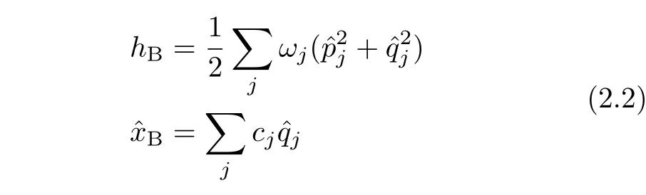
Throughout this paper we set~=1 and β=1/(kBT),with kBbeing the Boltzmann constant and T the temperature. Adopt the dimensionless solvation coordinate,in Eq.(2.2).Let≡an average over the bare bath thermal equilibrium ensembles.The effective system Hamiltonian,as inferred from Eq.(2.1),would assume

DenoteSet hereafter t≥0 for the time variable,unless further specified.

It is worth noting that Eq.(2.1)is just one prescription of the total composite Hamiltonian,with the specified reference bath of hB.In the presence of nonlinear coupling bath,different reference bath Hamiltonians are no longer mirror image to each other.It requires that the total composition HTbe of the prescription invariance,with difference reference bath Hamiltonians.Moreover,the characterization on the coupling bath α-parameters in Eq.(2.1),including α0for the energy reorganization,goes beyond the linear response theory.Physically supported models would be needed to complete the characterization of the α-parameters[20,21];see Section IV for further elaborations.

It is also noticed that the solvation coordinate,as described in Eq.(2.2),is a macroscopic bath degree of freedom.It couples directly to the system dissipative mode,,and meanwhile it is subject to a Brownian motion in the secondary bath environment.In contract to the DEOM theory in Section III,the extended FP-QME to be developed in Section IV describes the Brownian motion explicitly.In principle,one can have the“core-DEOM”theory,with the linear coupling secondary environment.However,this approach is much more expensive in general,as it accesses also the dynamics of the secondary dissipatons.We will see later that the effects of nonlinear coupling bath could be taken into account via the generalized Wick’s theorem(cf.Section III.B).

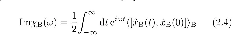
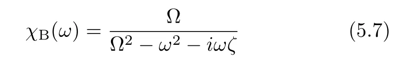
Turn to the characterization of dissipatons.These are statistical quasi-particles,defined via the linear solvation correlation function in the bare bath ensembles at thermal equilibrium[17–19].Let χB(ω)be the Laplace frequency resolution of the solvation response function.Its real part is symmetric and imaginary part is antisymmetric.The latter reads[14]

This defines the solvation bath spectral density,in agreethe microscopic formula following directly from Eq.(2.2).Together with the detailed-balance relation,Eq.(2.4)leads to[14]

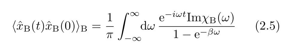
This is the fluctuation-dissipation theorem[13–16].The time-reversal relation for correlation functions reads[14]

To proceed,we exploit a certain efficient and accurate sum-over-poles scheme[32,33]to decompose the Fourier integrand in Eq.(2.5),followed by the Cauthy’s contour integration in the lower-half plane.We obtain

It is easy to show that(i)the individual exponential term arising from the Bose function is real,and(ii)those{γk}arising from the spectral density function are either real or complex conjugate-paired[8,18].In other words,the associate index,¯k,defined via γ¯k≡,must also appear in Eq.(2.7).We can therefore express the time-reversal counterpart to Eq.(2.7)via Eq.(2.6)as

The dissipaton decomposition on the solvation coordinate goes as follows,

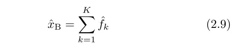
with

Apparently,both Eqs.(2.7)and(2.8)are satisfied.

As highlighted above,dissipatons consist of linear and statistically independent macroscopic degree of freedom,arising from the solvation coordinate.Each dissipaton goes by a single exponent,for its forward and backward correlation functions.This feature leads to[17,18]

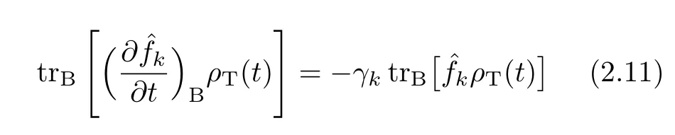
It will lead to the generalized diffusion equation in the DEOM theory,see Eq.(3.2).

III.DISSIPATON-EQUATION-OF-MOTION THEORY

A.Second quantization description

Dynamical variables in the DEOM theory are the socalled dissipaton density operators(DDOs)[17,18]:

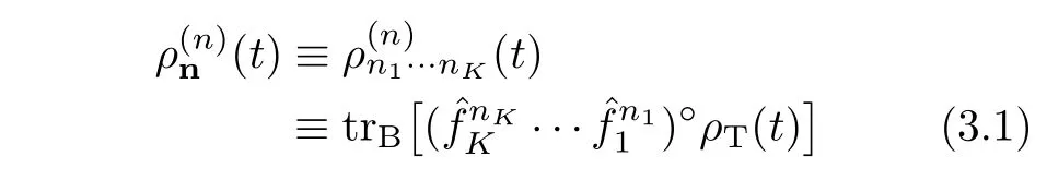
Here,n=n1+···+nK,with nk=0,1,2,···.The reduced system density operator is just ρS(t)≡ρ(0)(t).In general,(t)is an n-dissipatons DDO,with the configuration of n≡{n1···nK}that is an ordered set of occupation numbers on individual dissipatons.More precisely,the product of n-dissipatons inside the circled parentheses,(···)◦,is irreducible.It goes byfor Bosonic dissipatons that satisfy symmetric permutation.In other words,Eq.(3.1)resembles the second-quantization representation of a bosonic permanent.The DDOs with fermionic environment are similar,but resemble the Slater determinants,having the occupation numbers of 0 or 1 only,due to the antisymmetric permutation relation[17,18].The irreducibility notion,(···)◦,is also closely related to the generalized Wick’s theorem(cf.Section III.C).This is the most useful ingredient of the dissipaton algebra,which enables DEOM truly a type of“core-system”theory.Apparently,the DEOM space resembles a Fock space in quantum mechanics,with individual elements being the form of ρ(t)={(t);n=0,1,···,L}.Here,L denotes the converged many-dissipaton level.

The generalized diffusion equation,which dictates the influence of hBon DDOs without approximation,reads[17,18]

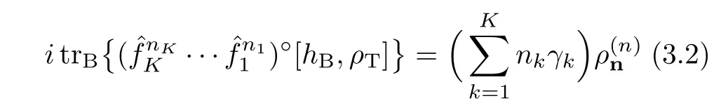
This is obtained via Eq.(2.11),together with the Heisenberg equation,and the trace cyclic invariance.It is noticed that in FP-QMEs,the influence of hBis described by the FP operator that involves a certain bi-dissipaton ansatz(cf.Section V.B).Equation(3.2)does generalize the eigenequation of the FP operator(cf.Eq.(6.18)).It resembles the secondquantization result on the influence of bare-bath hB.

B.The generalized Wick’s theorem

The generalized Wick’s theorem is the most important ingredient of the dissipaton algebra[17–21].It enables DEOM a theory for entangled system-and-bath dynamics[34–37],on top of the hierarchical dynamics an algebraic construction(cf.Section III.C).For bookkeeping,we denote the values of Eq.(2.10)at t→0+by

Moreover,the irreducibility notion,(···)◦in Eq.(3.1),facilitates the presentations below.

Generalized Wick’s Theorem-1(GWT-1)deals with the case of adding one dissipaton each time to DDOs of Eq.(3.1).For the forward action of a dissipaton,it reads[17,18]:

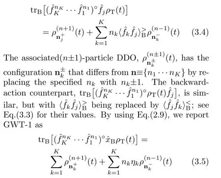
The backward-action counterpart is similar,but with ηkbeing replaced by.Apparently,GWT-1 deals with the linear coupling bath.

GWT-2 is concerned with the quadratic coupling bath,where a pair of dissipatons are added simultaneously each time.This would suggest that GWT-2 read[20,21]:

Thein the first term takes at the same time for the specified dissipatons pair that are added simultaneously.The associated DDO index,,differs from n≡{n1···nK}on the specified subindexes,nkand nj,that are replaced by nk±1 and nj±1,respectively.By using Eqs.(2.9)and(3.3),we can recast GWT-2 as

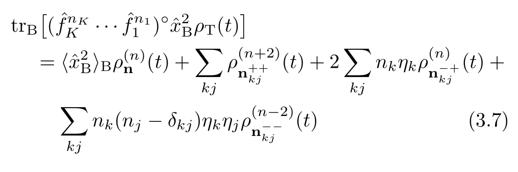
The backward-action counterpart is similar,but with ηkand ηjbeing replaced byrespectively.

C.Hierarchical dynamics equations

The complete DEOM theory consists also the hierarchical dynamics formalism for DDOs.Let us start with the time derivative on Eq.(3.1),

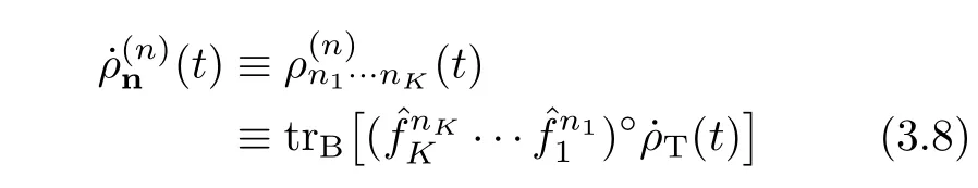
where(t)=−i[HT,ρT(t)].We evaluate Eq.(3.8)with the each individual term in the total system-and-bath composite HTof Eq.(2.1).While the generalized diffusion Eq.(3.2)has taken care of the bath hBaction,the generalized Wick’s theorem is the vehicle to the algebraic evaluation on the influence of system-coupling bath.In particular,GWT-1 and GWT-2,Eqs.(3.5)and(3.7)and their backward-action counterparts,evaluate the influences of linear and quadractic coupling bath,respectively.Apparently,⟩Bin the first term of Eq.(3.7)enters into the effective system Hamiltonian,HSeffof Eq.(2.3).

The final hierarchical dynamics formalism reads

In the absence of quadratic coupling(α2=0),Eq.(3.9)reduces to the HEOM formalism[3–6].The latter is a path integral influence functional based theory[1],withbeing considered as mathematical auxiliaries.The above observations validate the generalized diffusion Eq.(2.11)that leads to Eq.(3.2),and GWT-1,Eq.(3.4)or Eq.(3.5),and the time-reversal counterpart.While the conventional diffusion equation[38]and Wick’s theorem[14,15]are concerned only with C-number properties of Gaussian statistics,those two generalizations,Eqs.(2.11)and(3.4),go with reduced operators in the system-subspace,with arbitrary Hamiltonian HSand arbitrary dissipative modeˆQS.

Nevertheless,GWT-2,Eq.(3.6)or Eq.(3.7),is subject to further scrutiny.Analytically,we had validated it in the high-temperature regime[20];however,numerically,we found it would be only applicable up to a moderate strength of quadratic coupling bath[21].The above observations would suggest that Eq.(3.7)would be a sort of Ehrenfest mean- field treatment on quadratic coupling bath[21].We will defer this issue to future study.

IV.THEORY OF NONLINEAR COUPLING BATH DESCRIPTORS

To complete the quantum dissipation theory with nonlinear coupling environments,we shall further have physically supported α-parameters in Eq.(2.1).It is well known that in the presence of quadratic coupling bath,the α-parameters cannot be characterized solely via the linear response theory.Additional information is needed.

In the follow we present an extended solvation model approach to the required linear-plus-quadratic coupling bath descriptors[21].Let us examine the systembath interaction,the last term of Eq.(2.1).Physically it arises from the surrounding environment rearrangements in response to the dissipative system operatorˆQS.The solvation model approach is to rewrite Eq.(2.1)as

with

Meanwhile,we examine the reference-bath invariance requirement by recasting the last two terms of Eq.(4.1)as

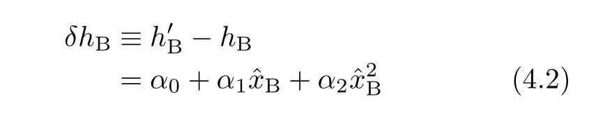
This identity relates between the reference-hBand the reference-based descriptions,with δhB≡−hBbeing given by Eq.(4.2),whereas

We can then recast Eq.(4.3)in terms of

Here the primed quantities and unprimed ones are associated with the-and the hB-based prescriptions,respectively.This follows the spectroscopic notation,as ifand hBwere the molecular nuclear Hamiltonians associated with electronic excited and ground states,respectively[39,40].Apparently,the linear and quadratic terms arise from the linear displacement and frequency shift,respectively;i.e.,

To proceed,let us divide the overall bath,hB,into the solvation mode and secondary bath parts.In line with the complete square-form of hBin Eq.(2.2),its partition would read[27,28]

As implied here the solvation mode is subject to a Brownian oscillator motion in the secondary bath,withThe latter gives rise to the stochastic random force:

and also the associated friction kernel:

on the solvation mode.The Langevin equation reads

Together within Eq.(2.4)the expression[14,15],

with the complex friction function,

It is also easy to obtain[14]

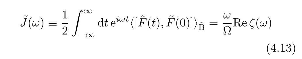
The first identity defines the secondary interacting bath spectral density(cf.Eq.(2.4)).Applying Eq.(4.11)for Eq.(4.13)leads to˜ωJ(ω)=ImχB(ω)/|χB(ω)|2.This is the relation between the secondary interacting bath spectral density and that of the overall one[14,23].The interacting secondary bath correlation function reads[cf.Eq.(2.5)]

Apparently,the complete characterization requires not only the α-parameters,but also χB(ω)of Eq.(4.11),as inferred from Eq.(2.5).

The expression ofis similar to Eq.(4.7),but with primed quantities.Thebath coordinates are given bywith respect to their reference hB-based counterparts.However,as elaborated in Ref.[21],the physical model for Eqs.(4.2)or(4.4)implies that the secondary bath environments do not contribute the quadratic coupling,i.e.,,but only the linear displacements.It also requires that the effects of secondary bath be representable with the solvation coordinatexˆ only,on the basis of a set of well defined linear displacement mapping rules[21].This is achievable when the radio,,between the coupling bath strength parameter inand that in hBof Eq.(4.7),can be effectively replaced by a single kindependent polarization constant[21].This undetermined constant actually dictates the reference-based ζ′(ω),with respect to the hB-based ζ(ω)of Eq.(4.12)with Eq.(4.9).The characterization is then carried out by using explicitly the prescription requirement,as described by Eqs.(4.2)–(4.6).

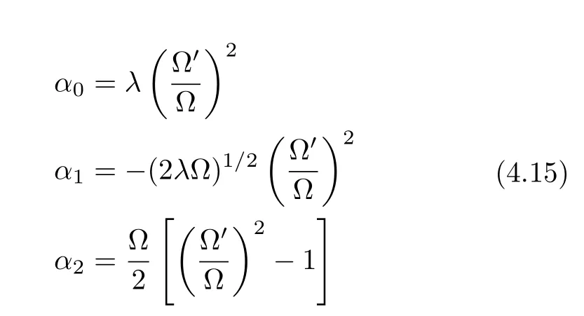
The final results in the hB-based prescription read[21]

Here,λ≡Ωd2/2 denotes the reorganization energy,due to the linear displacement in Eq.(4.6),whereas d2/2 amounts to the Huang-Rhys factor.

The-based counterparts read[21]

Meanwhile we have also identified the aforementioned polarization constant to be ofIt gives rise to have ζ′(ω)=ζ(ω),the same as that of the reference hB-based prescription.The-based counterpart to Eq.(4.11)is therefore[21]

The required nonlinear coupling bath descriptors are now completed.

V.EXTENDED FOKKER-PLANCK QUANTUM MASTER EQUATION

A.Remarks on quantum versus semiclassical bath

It is worth reemphasizing that both the DEOM and FP-QME are“core-system”dynamics theories.While the former reveals the solvation dynamics via generalized Wick’s theorem,the latter deals explicitly with the reduced core-system density operator.Here,the overall bath hBof Eq.(2.2)is divided into two parts as Eq.(4.7):the solvation mode,/2,and the interacting secondary bath part,denoted as hB˜Bbelow.The total composite Hamiltonian,Eq.(2.1),can be recast as

with(noting that HS≡H0+α0ˆQSas Eq.(2.3))

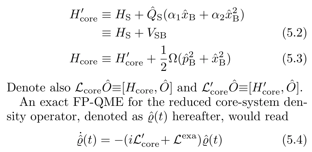
with the quantum Fokker-Planck operator of

One can investigate Lexain the absence of the primary system.This would be equivalent to the Langevin equation(Eq.(4.10))for the Brownian dynamics of the solvation mode in the secondary bath.In general,the dissipative superoperator,ReBxa,depends on the initial condition on the total system-and-bath composite density operator[41,42].The resultant ReBxawould be quite complicated and also time-dependent[41,42].Nevertheless,the general expression goes beyond the scope of this paper,as our main interest is the underlying

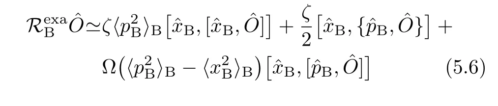
Here,ζ≃ζ(ω=0)denotes the effective friction constant;whereasand,the thermal equilibrium phase-space variances of the solvation mode in bare bath hB,are evaluated via Eq.(2.5)as

Some subtle issues arise in comparing the exact FPQME,Eqs.(5.4)–(5.6),to the approximated FP-QMEs that assume a Markov secondary bath,with ζ(ω)in Eq.(4.11)being replaced by the constant ζ;i.e.,

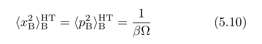
It is easy to show that in this casediverges[14,15].As inferred from Eq.(4.13),the Markov secondary bath is of˜J(ω)=ωζ/Ω.However,the resultant correlation funciton,⟨˜F(t)˜F(0)⟩˜βof Eq.(4.14),is not a white noise,unless assuming further the classical high temperature(HT)limit of

In this limit,

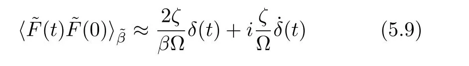
or

In this case,Eq.(5.6)reduces to

It leads to Eq.(5.4)the Caldeira-Leggett’s QME[27,28],

with(cf.Eq.(5.5))

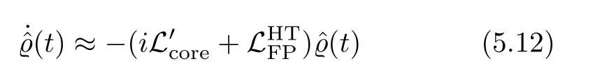
This is a mixed quantum-classical theory,with iLcorefor the coherent core-system dynamics,andfor the classical dissipative solvation dynamics in the secondary bath environment.However,as a classical bath theory,Eq.(5.12)is of a very limited applicability range in the parameters space.

It is anticipated that,as long as the coherent iLcoreand the incoherent RBare not treated at the same level,a certain caustic compensation would be required.This would give rise to an additional dissipative superoperator,δRSB,that depends explicitly on both the dissipative system and solvation bath modes.The resultant semiclassical FP-QME would assume the form of(see Section V.B)

The high-temperature limit,Eq.(5.12),is associated withof Eq.(5.13)and δ=0.

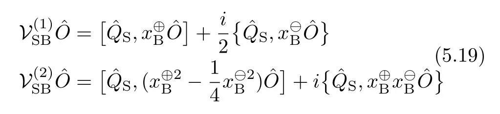
It would be insightful to have a close inspection on the incoherent δRSBcaustics versus the coherent interacting component ofthat reads(cf.Eq.(5.2))

Here,

To facilitate the later construction,we introduce

and similarlysuch that

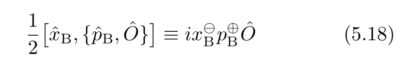
We can then express Eq.(5.16)as

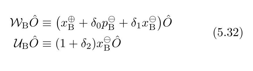
The caustic dissipation superoperator assumes also the form ofIt will be evident later that the final expressions(cf.Eqs.(5.30)–(5.32))can be conveniently expressed in terms of

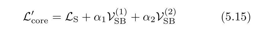
Recast now Eq.(5.14),with Eq.(5.15),as

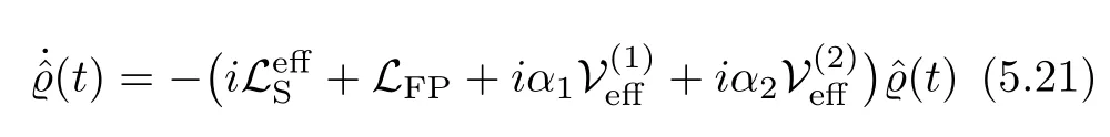
It is worth to mention that we usehere,instead of the presumed LS,as it would be if the exactor,Eq.(5.6),were used.Actually,the adopted LFPbelow(cf.Eq.(5.22))resembles formally as the high-temperature one,Eq.(5.13),withof Eq.(5.11).It does not have the-term,as in Eq.(5.6).A properormay partially makeup this loss.We adoptof Eq.(2.3),in line with the DEOM(Eq.(3.9)).

B.FP-QME with semiclassical bath

We will be interested in a semiclassical bath,having[30]

Formally it resembles Eq.(5.13)with Eq.(5.11);thus the well-established Fokker-Planck operator algebra[38]is directly applicable;see Section VI.A.Nevertheless,it replaces the solvation frequency and friction constant in Eq.(5.13)with temperature-dependent effective¯Ω and¯ζ.

More specifically,LFPof Eq.(5.22)goes by a bidissipaton(exponential)approximant of the solvation correlation function,Eq.(2.7),

where

Whileandare positive,η+and η−in Eq.(5.23)are complex.Parametrization goes with the so-called minimum-dissipaton ansatz[29]:

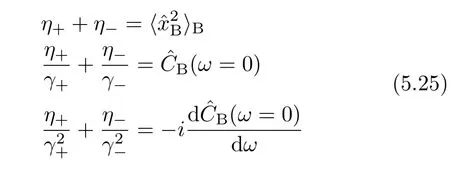
with the exact values via Eq.(2.5)on the left-hand-sides,where

Remarkably,for the Markovian Brownian osciallator of Eq.(5.7),one can analytically solve Eq.(5.25)and further identify its impressive accuracy range in the parameter space[29,30].One interesting result is that

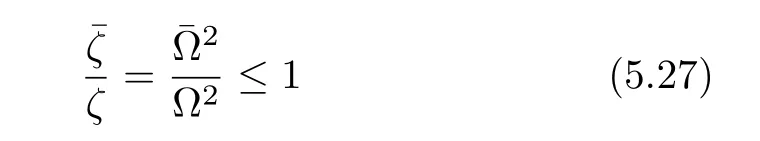
which can be recast in terms ofversus rBO≡ζ/(2Ω)asThe lower the temperature the smaller the ratio is,and the equal sign holds in the HT limit of T→∞only[29].

Introduce three real parameters,δ0,δ1and δ2,via[29,30]

Together with Eqs.(5.25)and(5.27),we obtain

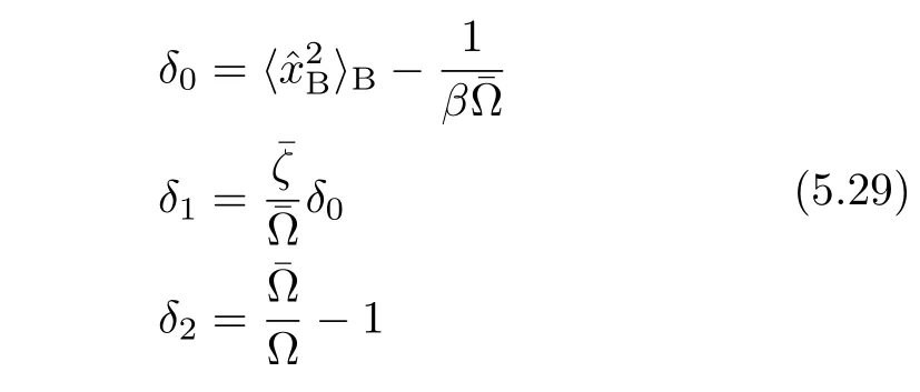
Physically,δ0and δ1are related to the short-time and long-time caustics,respectively,whereas δ2measures the caustic renormalization.These caustic parameters all vanish at the high-temperature limit.

The above semiclassical parametrization scheme was originally proposed in Ref.[29].It has also been used together with Eq.(5.22)in the construction of FP-QME(5.21)via its DEOM correspondence,in the absence of quadratic coupling bath[30].

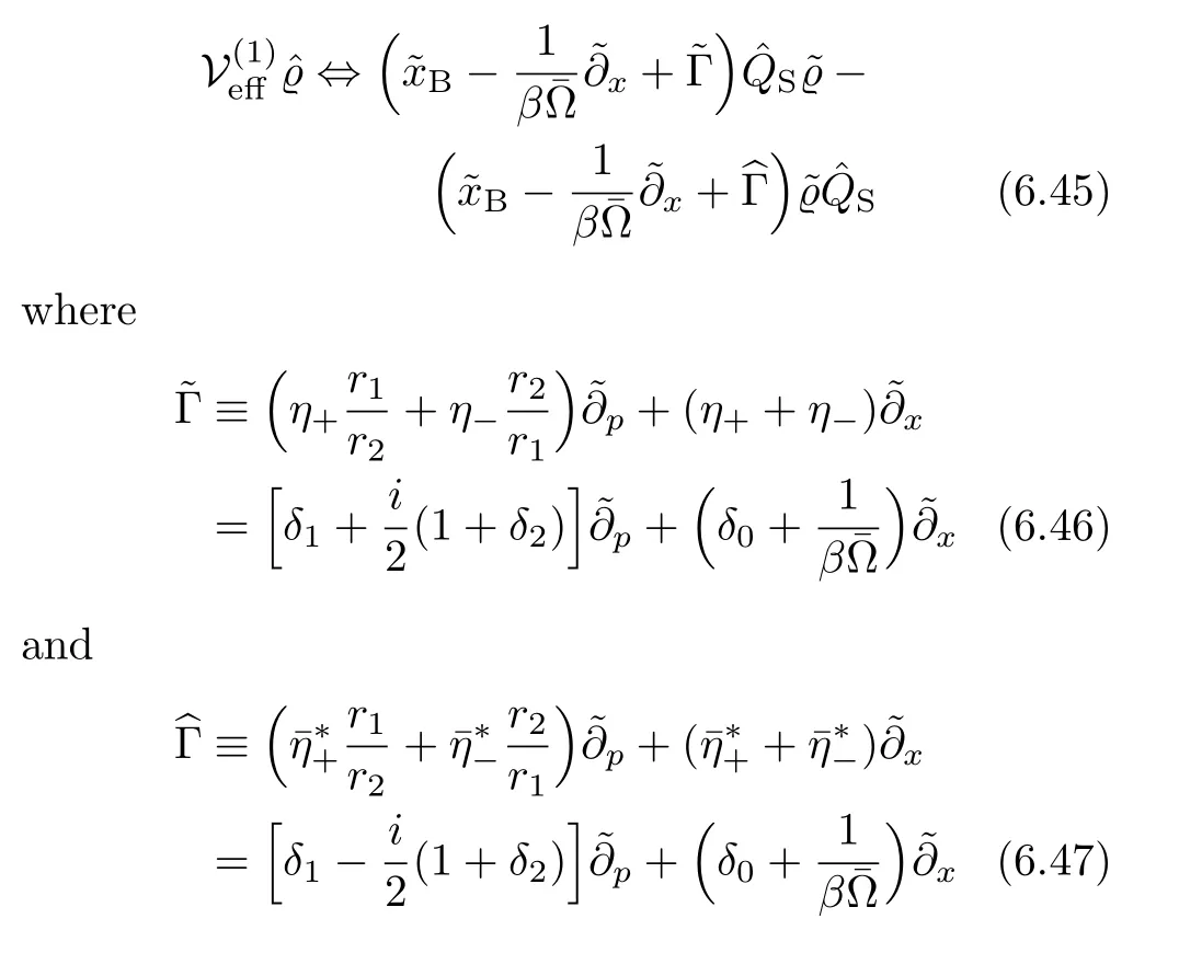
In this work,we apply the same construction method on Eq.(5.21)with the linear-plus-quadratic coupling bath.The final results read

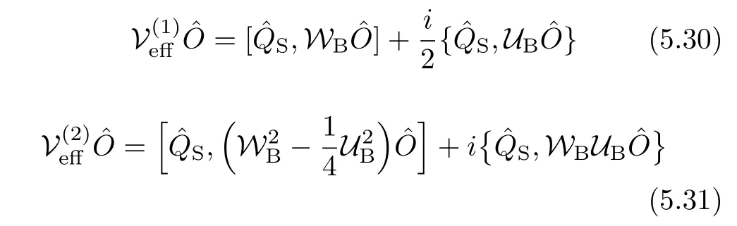
where

VI.FOKKER-PLANCK OPERATOR ALGEBRA VERSUS DISSIPATONS DYNAMICS

A.Fokker-Planck operator algebra

In this section,we derive the above FP-QME formalism,via its DEOM correspondence.The latter is just the bi-dissipaton version of Eq.(3.9);see Section VI.B for the details.Exploited will also be the Fokker-Planck operator algebra[38].The underlying quasiparticle picture will be elaborated in relation to that in Section III.

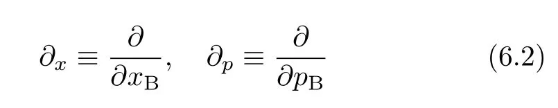
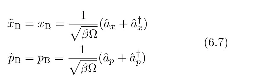
The derivations will be carried out in the Wigner representation for the solvation mode.While reduced core-systemremains an operator in the system subspace,the superoperators WBand UBin Eq.(5.32)become solvation phase-space operators;i.e.,

Here

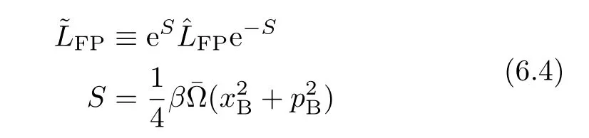
Meanwhile,LFP(Eq.(5.22))assumes the FP operator,

Its eigen solutions are analyzed via the similarity transformation,as follows[38].

Under this transformation,

where

We have

Apparently,It together with Eqs.(6.5)and(6.7)leads to Eq.(6.3)the S-transformed expression,

Note that

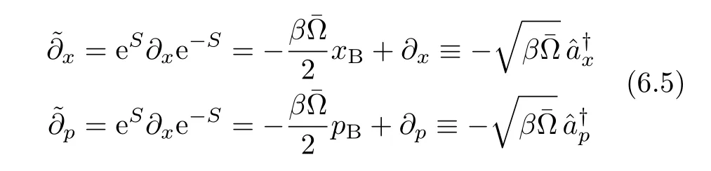
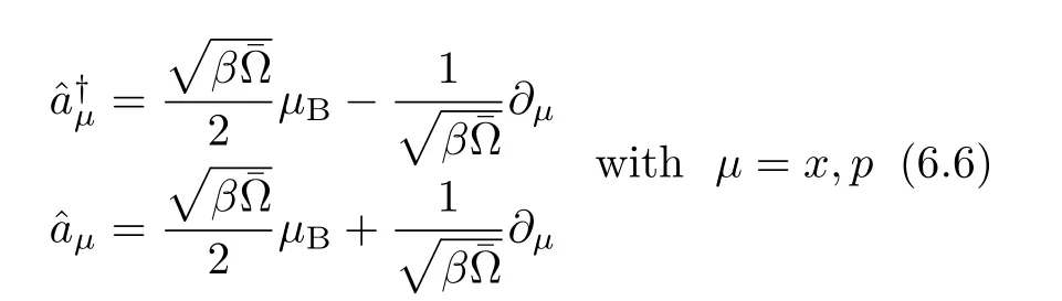
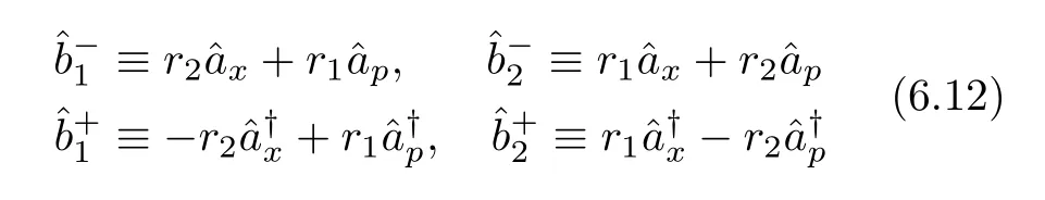
Introduce now the operators,;j=1,2,via

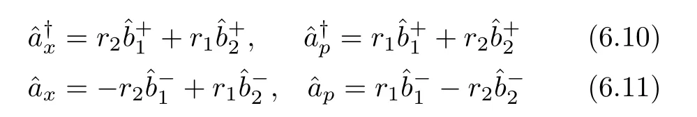
These are equivalent to

Despite of

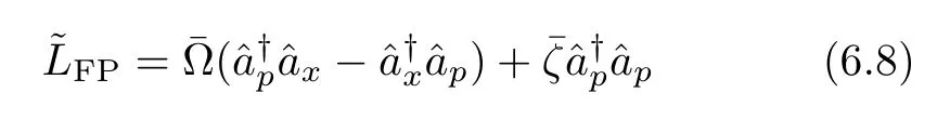
These lead to Eq.(6.8)the diagonalized form of

Due to the boson-like relations of Eq.(6.13),the standard harmonic oscillator algebra is applicable.We obtain

where nj=0,1,···,with the normalized ground state,

Further,fromobtain Eq.(6.14)the eigen solutions,

where

The physical implications on the above diagonalization will be discussed at the end of this subsection.

Introduce for the later use the scaled(unnormalized)eigenfunctions[30],

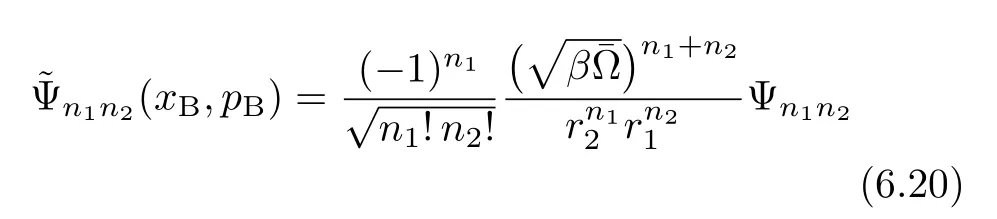
It is evident below that the phase-space actions on the scaled wavefunctions assume rather compact expressions.Forand(Eq.(6.5)),applying Eq.(6.10)and then Eq.(6.15),we obtain

Moreover,as the actions on the scaled eigenfunction are concerned,

where

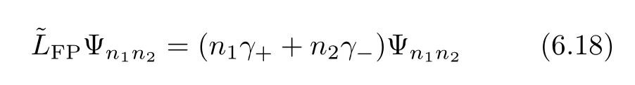
To conclude this subsection,we like to point out the implications on the above FP operator algebra.First of all,the eigen Eq.(6.18)resembles the generalized diffusion Eq.(3.2).It is noticed that the FP operator itself arises from the bare bath Hamiltonian hB;see Eq.(4.7)and also the comments following Eq.(5.5).Moreover,one can view Eq.(6.15)and Eq.(6.16)as the manifestation of the generalized Wick’s theorem,Eq.(3.4)the GWT-1.The effect of quadratic coupling bath on the eigenfunctions will resemble the GWT-2 Eq.(3.6).The above observations suggest the quasi-particle or dissipaton picture in the FP-QME.Nevertheless,the dissipaton approach provides much simpler algebra also clearer physical picture.

B.The corresponding dissipatons dynamics

To facility the later construction of FP-QME Eq.(5.21)via its DEOM correspondence,we present explicitly the bi-dissipaton version of Eq.(3.9),as follows.

The linear coupling bath related quantities are

and

The quadratic coupling bath engages

and

The superoperators involved in Eq.(6.25)follow those of Eq.(3.10);i.e.,

and

Note thatamounts to the pre-exponential coefficient η¯kof Eq.(2.8).As specified there,it can now be recast as

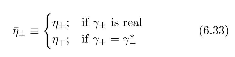
Moreover,as inferred from Eq.(5.23)and the time reversal relation,Eq.(2.6),we have

Taking the time derivative at t=0,we obtain

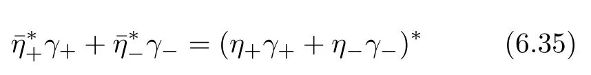
Together with(5.24)and(6.9);see also Eq.(5.28)),we have

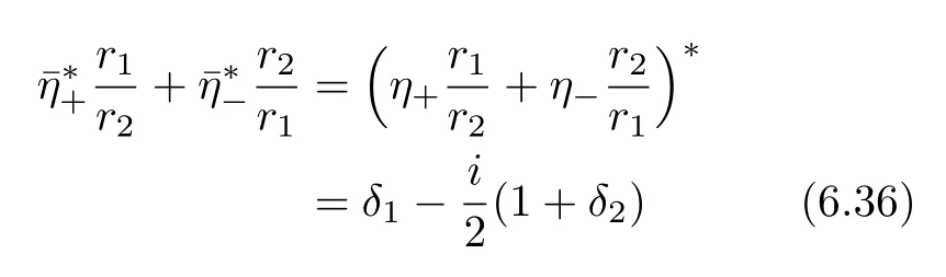
Together with Eq.(5.28),the above identities relate the complex η-parameters,in Eq.(6.31)and Eq.(6.32)of DEOM,to the real δ-parameters in Eq.(5.32)of FPQME.

C.The FP-QME space verse the DEOM space

We can now complete the construction of FPQME(5.21),with Eq.(5.30)−Eq.(5.32)based on its DEOM counterpart,Eq.(6.25)−Eq.(6.32).Let ˜ϱ(xB,pB,t)≡eSˆϱ(xB,pB,t),the same similarity transformation used in the LP operator diagonalization;cf.Eq.(6.4).The construction starts with

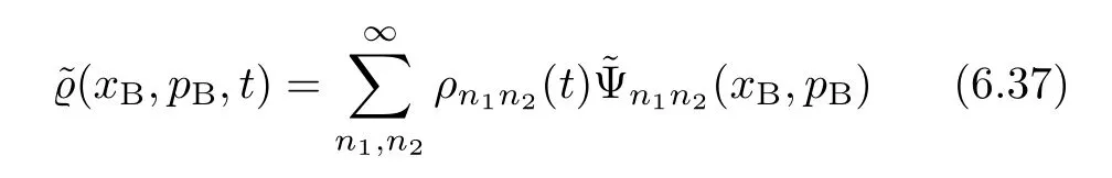
This variables-separation expression specifies the fact that the FP-QME dynamics is identical to its DEOM counterpart DEOM2.The expansion basis set,{(xB,pB)},specified in Eq.(6.20),are those properly scaled eigenfunctions of the LP operators,as we did before for the linear coupling case[30].

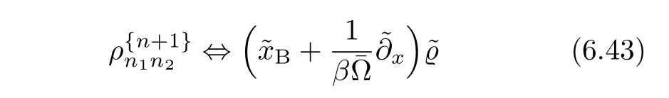
In the following derivations,we adopt the notation of correspondence,“⇔”,in which Eq.(6.37)reads

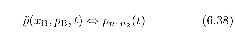
Apparently,it would also lead to the operator-level correspondence of(t)⇔ρn1n2(t).

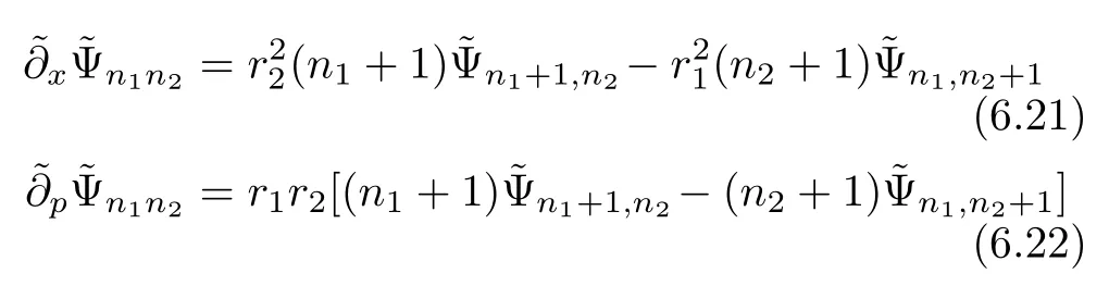
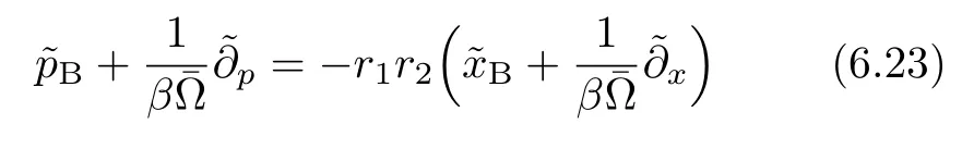
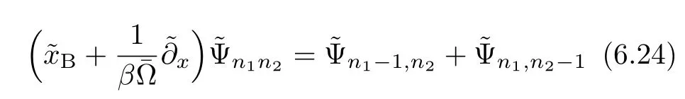
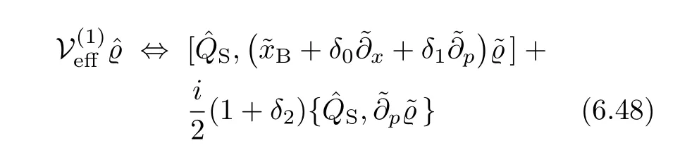
The phase-space actions on(xB,pB,t),as involved in Eq.(6.1),can now be carried out easily,by using Eq.(6.21)−Eq.(6.24).For example,Eq.(6.24)results in

Following the notation that defines Eq.(6.38)for Eq.(6.37),the last expression above reads

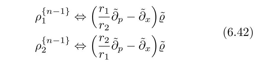
Similarly,we have

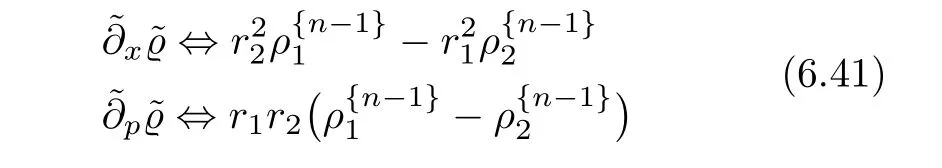
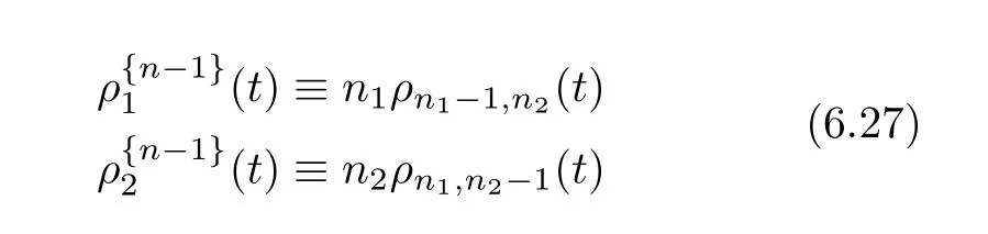
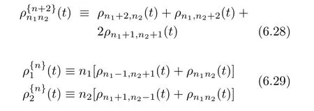
The involvedwere defined in Eq.(6.27).The solutions here are

Moreover,by using Eq.(6.26),we recast Eq.(6.40)as

Now comparing the linear coupling bath contribution,the α1-term in Eq.(6.25),with that in Eq.(5.21),we have

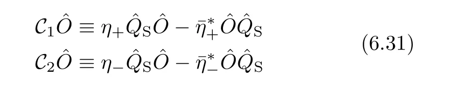
Applying AˆO≡[ˆQS,ˆO]and Eq.(6.31)for C-actions on the specified operators,with Eq.(6.42)and Eq.(6.43),we obtain

The second identity in each of the above two equations is obtained by using Eq.(6.36)and alsoη−;see Eq.(5.28).We can then rearrange Eq.(6.45)as

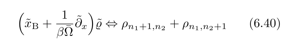
By applying Eq.(6.1),we obtain

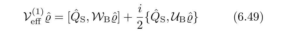
This is just Eq.(5.30).

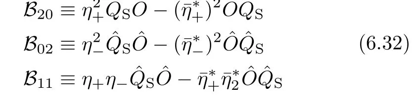
The influence of the quadratic coupling bath can be treated similarly,as follows.By comparing between the α2-term in Eq.(6.25),and that in Eq.(5.21),we have

Apparently,the evaluations involve double-actions of linear operators in the Wigner phase-space.In specific,the double-action of Eq.(6.40)or Eq.(6.43)would lead to

Moreover,by applying the phase-space action in Eq.(6.43),followed by each individual in Eq.(6.42),we obtain

Furthermore,the pairs action in Eq.(6.42)result in

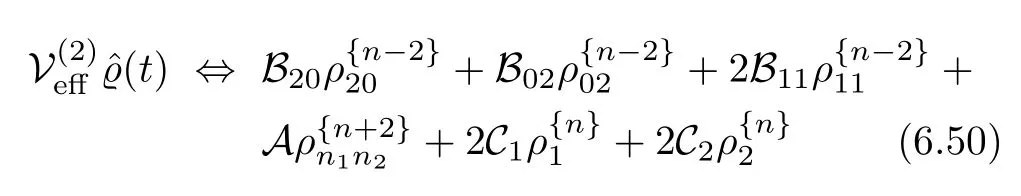
By applying the same procedure,as from Eq.(6.44)to Eq.(6.49),we obtain Eq.(6.50)the expression,

This is just Eq.(5.31).We have thus completed the construction of FP-QME(5.21),with Eqs.(5.30)–(5.32).

VII.CONCLUDING REMARKS

In summary,we present a comprehensive account on the theories of quantum open system,with quadratic coupling bath environments.It is worth to reemphasize that even the nonlinear coupling bath characterization itself is nontrivial.The results presented in Section IV just represent one of physically supported schemes.

Both the DEOM and FP-QME approaches to the entangled system-and-environment dynamics are presented and scrutinized,with the focus on the underlying quasi-particle picture.Apparently,the DEOM approach enjoys a much clearer physical picture and much more friendly use in evaluating various systems.Nevertheless,the extended FP-QME,which is developed in this work,is carried out with a rather straightforward algorithm.The underlying equivalence between these two dynamics approaches would shed some light on the advancement of the DEOM theory with nonlinear coupling bath environments.

VIII.ACKNOWLEDGEMENTS

This work was supported from the Ministry of Science and Technology(No.2016YFA0400900),the National Natural Science Foundation of China(No.21373191,No.21633006,and No.21303090),and the Fundamental Research Funds for the Central Universities(No.2030020028).

[1]R.P.Feynman and F.L.Vernon Jr.,Ann.Phys.24,118(1963).

[2]J.S.Jin,X.Zheng,and Y.J.Yan,J.Chem.Phys.128,234703(2008).

[3]Y.Tanimura,Phys.Rev.A 41,6676(1990).

[4]Y.Tanimura,J.Phys.Soc.Jpn.75,082001(2006).

[5]R.X.Xu,P.Cui,X.Q.Li,Y.Mo,and Y.J.Yan,J.Chem.Phys.122,041103(2005).

[6]J.J.Ding,R.X.Xu,and Y.J.Yan,J.Chem.Phys.136,224103(2012).

[7]Y.A.Yan,F.Yang,Y.Liu,and J.S.Shao,Chem.Phys.Lett.395,216(2004).

[8]R.X.Xu and Y.J.Yan,Phys.Rev.E 75,031107(2007).

[9]J.S.Shao,J.Chem.Phys.120,5053(2004).

[10]J.M.Moix and J.S.Cao,J.Chem.Phys.139,134106(2013).

[11]Y.L.Ke and Y.Zhao,J.Chem.Phys.145,024101(2016).

[12]Y.L.Ke and Y.Zhao,J.Chem.Phys.146,174105(2017).

[13]R.Kubo,M.Toda,and N.Hashitsume,Statistical Physics II:Nonequilibrium Statistical Mechanics,Berlin Heidelberg:Springer-Verlag,(1991).

[14]Y.J.Yan and R.X.Xu,Annu.Rev.Phys.Chem.56,187(2005).

[15]U.Weiss,Quantum Dissipative Systems,4th Edn.Singapore:World Scientific,(2012)

[16]H.Kleinert,Path Integrals in Quantum Mechanics,Statistics,Polymer Physics,and Financial Markets,5th Edn.,Singapore:World Scientific,(2009).

[17]Y.J.Yan,J.Chem.Phys.140,054105(2014).

[18]Y.J.Yan,J.S.Jin,R.X.Xu,and X.Zheng,Frontiers Phys.11,110306(2016).

[19]H.D.Zhang,R.X.Xu,X.Zheng,and Y.J.Yan,Mol.Phys.116,780(2018).

[20]R.X.Xu,Y.Liu,H.D.Zhang,and Y.J.Yan,Chin.J.Chem.Phys.30,395(2017).

[21]R.X.Xu,Y.Liu,H.D.Zhang,and Y.J.Yan,J.Chem.Phys.148,114103(2018).

[22]A.A.Golosov,R.A.Friesner,and P.Pechukas,J.Chem.Phys.112,2095(2000).

[23]M.Thoss,H.B.Wang,and W.H.Miller,J.Chem.Phys.115,2991(2001).

[24]A.Garg,J.N.Onuchic,and V.Ambegaokar,J.Chem.Phys.83,4491(1985).

[25]L.D.Zusman,Chem.Phys.49,295(1980).

[26]L.D.Zusman,Chem.Phys.80,29(1983).

[27]A.O.Caldeira and A.J.Leggett,Ann.Phys.149,374(1983),[Erratum:153,445(1984)].

[28]A.O.Caldeira and A.J.Leggett,Physica A 121,587(1983).

[29]J.J.Ding,H.D.Zhang,Y.Wang,R.X.Xu,X.Zheng,and Y.J.Yan,J.Chem.Phys.145,204110(2016).

[30]J.J.Ding,Y.Wang,H.D.Zhang,R.X.Xu,X.Zheng,and Y.J.Yan,J.Chem.Phys.146,024104(2017).

[31]H.Liu,L.L.Zhu,S.M.Bai,and Q.Shi,J.Chem.Phys.140,134106(2014).

[32]J.Hu,R.X.Xu,and Y.J.Yan,J.Chem.Phys.133,101106(2010).

[33]J.Hu,M.Luo,F.Jiang,R.X.Xu,and Y.J.Yan,J.Chem.Phys.134,244106(2011).

[34]J.S.Jin,S.K.Wang,X.Zheng,and Y.J.Yan,J.Chem.Phys.142,234108(2015).

[35]H.D.Zhang,R.X.Xu,X.Zheng,and Y.J.Yan,J.Chem.Phys.142,024112(2015).

[36]H.D.Zhang,Q.Qiao,R.X.Xu,and Y.J.Yan,Chem.Phys.481,237(2016).

[37]H.D.Zhang,Q.Qiao,R.X.Xu,and Y.J.Yan,J.Chem.Phys.145,204109(2016).

[38]H.Risken,The Fokker-Planck Equation,Methods of Solution and Applications,2nd Edn.,Berlin:Springer-Verlag,(1989).

[39]S.Mukamel,The Principles of Nonlinear Optical Spectroscopy,New York:Oxford University Press,(1995).

[40]Y.J.Yan and S.Mukamel,J.Chem.Phys.85,5908(1986).

[41]B.L.Hu,J.P.Paz,and Y.Zhang,Phys.Rev.D 45,2843(1992).

[42]R.X.Xu,B.L.Tian,J.Xu,and Y.J.Yan,J.Chem.Phys.130,074107(2009).

[43]R.X.Xu,Y.Mo,P.Cui,S.H.Lin,and Y.J.Yan,inProgress in Theoretical Chemistry and Physics,Vol.12:Advanced Topics in Theoretical Chemical Physics,J.Maruani,R.Lefebvre,and E.Brändas,Eds.Dordrecht:Kluwer,7–40(2003).