Fast Solving the Cauchy Problems of Poisson Equation in an Arbitrary Three-Dimensional Domain

Cheinshan Liu, Fajie Wang and Wenzheng Qu

1 Introduction

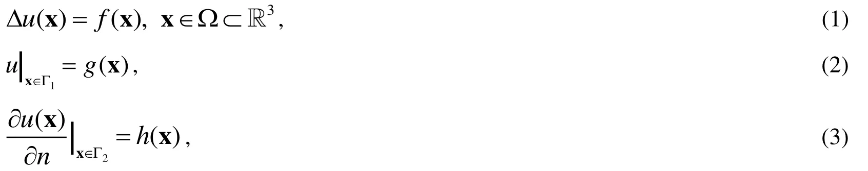
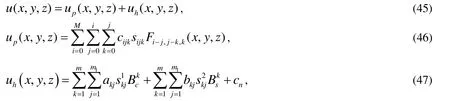
In this paper we propose a new two-stage method to solve the following three-dimensional Poisson equation:

Liu [Liu (2008a)] has applied a modified Trefftz method (TM) to recover the unknown boundary data for the inverse Cauchy problem, but one needs to consider a regularization technique by truncating the higher-mode components of the given data. Then, Liu [Liu(2008b)] employed the modified collocation Trefftz method with a single characteristic length to solve the inverse Cauchy problems in simply and doubly-connected domains. Liu[Liu (2012b)] has developed a very powerful optimally generalized regularization method to solve the Cauchy problem of Laplace equation by using the method of fundamental solutions (MFS). Up to now, most researches are restricted in the two-dimensional inverse Cauchy problems [Fan, Li and Yeih (2015)]. Only a few studies the inverse Cauchy problem in three- or higher-dimensional cases [Wei, Hon and Cheng (2003); Wang, Chen,Qu et al. (2016)].

There are many papers dealing with the numerical solutions of elliptic type partial differential equations (PDEs). Presently, the method that uses point collocation rather than mesh with weighted integration appears as an effective method, which includes the MFS[Golberg (1995)], the Trefftz method [Li, Lu, Huang et al. (2007); Li, Lu, Hu et al. (2008)]and the radial basis function (RBF) collocation method [Kansa (1990)]. Li et al. [Li, Lu,Hu et al. (2008)] gave a very detailed description of the collocation Trefftz method. The meshless and mesh reduction methods are nowadays the main trend of numerical solution methods of boundary value problems (BVPs) [Liu (2007); Liu (2008b); Pradhan, Shalini,Nataraj et al. (2011); Zhu, Zhang and Atluri (1999); Atluri and Zhu (1998); Atluri, Kim and Cho (1999); Atluri and Shen (2002); Cho, Golberg, Muleshkov et al. (2004); Qu, Chen and Fu (2015); Jin (2004); Li, Lu, Huang et al. (2007)]. Many collocation techniques with the expansion of trial solutions by different basis-functions were employed to solve the elliptic type BVPs; see, for example, [Cheng, Golberg, Kansa et al. (2003); Hu, Li and Cheng (2005); Algahtani (2006); Tian, Reutskiy and Chen (2008); Hu and Chen (2008);Libre, Emdadi, Kansa et al. (2008)].

In order to overcome the ill-posed linear systems by using the Trefftz method, Liu et al.[Liu, Yeih and Atluri (2009)] have developed a multi-scale Trefftz-collocation Laplacian conditioner. The concept of multi-scale Trefftz-collocation method has been later employed by Chen et al. [Chen, Yeih, Liu et al. (2012)] to solve the sloshing wave problem.Liu et al. [Liu and Atluri (2013)] have employed the concept of equilibrated matrix to find the best multiple-scale of the Trefftz method used in the solution of the inverse Cauchy problems for the Laplace equation, whose resulting linear system is less ill-conditioned.The meshless methods, however, only solve the homogeneous PDEs. For nonhomogeneous PDEs, a special technique of particular solution is often used to remove the right-hand side,such that the usual MFS, TM and RBF can be applied. It is a key point to find the particular solution of PDEs for the nonhomogeneous problems. The method of particular solution(MPS) is popular in the text book for solving the nonhomogeneous PDEs. In general, we cannot find a global closed-form particular solution for an arbitrary right-hand side.However, for certain function bases, each term in the bases may have a corresponding closed-form particular solution [Cheng (2000); Golberg, Muleshkov, Chen et al. (2003);Chen, Fan and Wen (2012); Lamichhane and Chen (2015)].

In this paper, we will solve the Poisson equation by a two-stage method: first the particular solution and then the Laplace equation by using, respectively, the multiple-scale polynomial method and the multiple/scale/direction Trefftz method. The multiple/scale/direction Trefftz method was first developed by Liu [Liu (2016)] to solve the inverse Cauchy problem of 3D Helmholtz equation, and then Liu et al. [Liu, Qu, Chen et al. (2017)] solved the inverse Cauchy problem of 3D modified Helmholtz equation. This method reducing the number of Trefftz bases for 3D problems is a novel technology, which is not yet applied to solve the inverse Cauchy problem of nonhomogeneous PDE, like the 3D Poisson equation. Besides that, the present paper possesses another novelty by using the multiple-scale technique to interpolate 3D data, which is not yet reported in the literature.

The remainder of this paper is arranged as follows. In Section 2, we introduce a two-stage method and a multiple-scale polynomial method for the interpolation of given data. In Section 3, we find a particular solution, and review the Trefftz method endowing with a set of the Trefftz T-complete bases for the two- dimensional Laplace equation, which is extended to the multi-dimensional Trefftz method for solving the multi-dimensional Laplace equation. In Section 4.1, the numerical examples for the direct problems are given,while the numerical examples for the inverse Cauchy problems are given in Section 4.2.Finally, we draw conclusions in Section 5.

2 A two-stage method

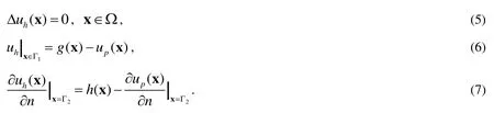
but does not satisfy the boundary conditions (2) and (3) necessarily. Hence, the problem(1-3) reduces to solve a homogeneous equation through

Usually, Eq. (9) is an over-determined system for that we may collocate more points to generate more equations with number, which are used to findcoefficients inwithHere the dimension ofis

An equilibrated matrix has either the same norm of all columns or the same norm of all rows, and under this condition the matrix is better-conditioned than that without considering the scaling technique. The problem is the search of some suitable matricesand, such that the condition number ofis significantly reduced. Liu [Liu (2013)]has proposed a simple procedure to find diagonalandonly through a few operations.

Liu [Liu (2012a)] has used the concept of equilibrated matrices to choose the best source points for the method of fundamental solutions, while according to the idea of equilibrated matrix, Liu [Liu (2012b)] has developed a general purpose optimally scaled vector regularization method to treat the ill-conditioned linear problems.

The scales are determined below, which are used to reduce the condition number of the new coefficient matrix, such that we can quickly find the expansion coefficients. If the norm of each column of the new coefficient matrix ofis required to be equal, the multiple-scaleis obtained fromvia a vectorization, is determined by

We can introduce a post-conditioning matrixby

such that the above equilibrated multiple-scale technique is equivalent to derive the new coefficientby

Instead of Eq. (11), we can solve a normal linear system:

where

The conjugate gradient method (CGM) is a powerful solution scheme and can be employed here to solve Eq. (14), the calculation steps of this method are summarized as follows:

(ii) Repeat the following steps for

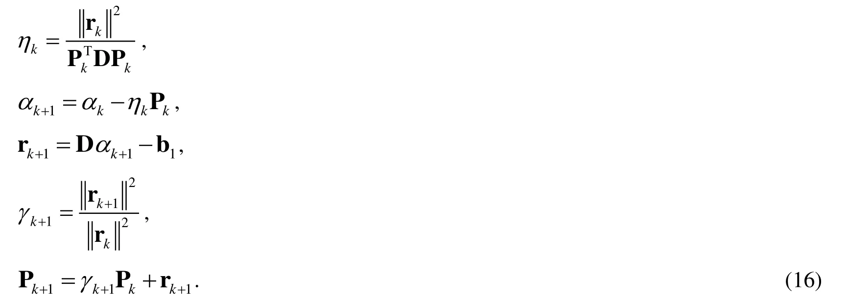
Until a given stopping criterionis satisfied, then stop.

We give two examples for the data interpolation by using the above multiple-scale polynomial method (MSPM).

Examples 1 and 2.We interpolate two given functions:

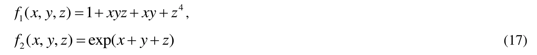
where

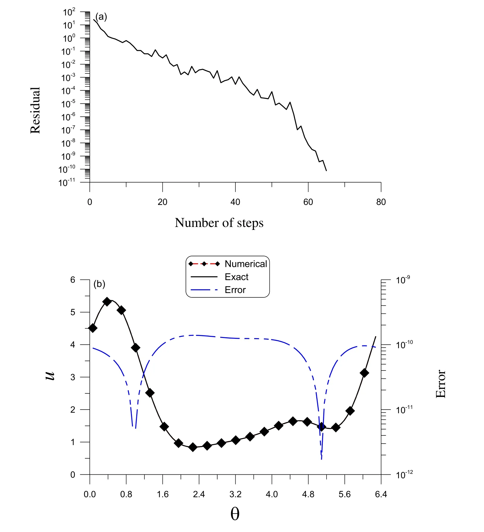
Figure 1: For example 1 of a 3D interpolation in an irregular domain, (a) convergence rate,and (b) the comparison of the numerical and exact solutions. The numerical and exact solutions overlap, such that the difference is not visible in the figure

Figure 2: For example 2 of a 3D interpolation of a complex function in an irregular domain,(a) convergence rate, and (b) the comparison of the numerical and exact solutions. The numerical and exact solutions overlap, such that the difference is not visible in the figure

3 A multi-dimensional Trefftz method

3.1 Particular solution

Although upin Eq. (20) is not a closed-form particular solution, but each term in upis a closed-form solution. By inserting the above upinto Eqs. (6) and (7), the right-hand sides can be obtained. Now a remained problem is how to solve Eqs. (5-7).

3.2 The Trefftz method

We first consider the following two-dimensional Laplace equation:

which are polar coordinates in the Euclidean spaceEq. (22) can be rewritten as

It is well-known that for an interior problem of two-dimensional Laplace equation,

forms a set of complete Trefftz bases [Liu (2007); Liu (2008b)].

Now, the Trefftz method based on the above bases (26) for the two-dimensional Laplace Eq. (22) can be written as

3.3 The multiple-scale-direction Trefftz method

In order to solve the multi-dimensional Laplace equation, we extend the result in Section 3.2 to a multi-dimensional case. Let

which is recast to

Let

where

We introduce

As mentioned in Section 3.2 we have the bases

which satisfy the two-dimensional Laplace equation in terms of:

We can expand the trial solution ofby

by summing the above equation with respect to i forEq. (34), we have

Inserting Eq. (42) into Eq. (38) we have

Thus, it has been proved thatsatisfies the q-dimensional Laplace Eq. (30). Similarly, it can be proved thatsatisfies the q-dimensional Laplace Eq. (30). Consideringdifferent directions in space, the expansion in Eq. (40) is called a multiple/scale/direction Trefftz method (MSDTM), of which the multiple scalesandare determined by the boundary collocation points as that in Section 2.

Ku et al. [Ku, Kuo, Fan et al. (2015)] have employed the multiple-scale Trefftz method withindependent bases of the Bessel functions and the modified Bessel functions expressed in the cylindrical coordinates to solve the three-dimensional Laplacian problems.In detail, it expands the solution by

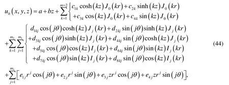
It can be seen that the MSDTM is simpler than that of the above standard Trefftz method [Ku,Kuo, Fan et al. (2015)], where many tedious works to establish the bases functions are necessary. When the number of unknown coefficients of MSDTM isthat of the standard Trefftz method is aboutLater, the above bases have been used to solve the 3D Laplace equation and compared it with the MFS [Lv, Hao, Wang et al. (2017)].

4 Numerical tests

Encouraged by the accuracy in the data interpolation, we will further combine the multiplescale polynomial method and the multiple /scale/direction Trefftz method to solve the Poisson equation, including the direct problem and the inverse Cauchy problems.

4.1 Direct problems

Example 3.First, we consider the Poisson equation as follows:

in which

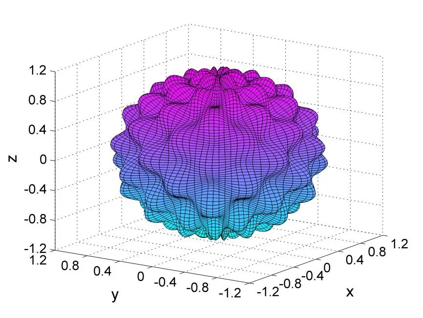
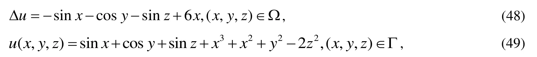
Figure 3: Irregular domain for example 3

The particular solution is obtained by using the MSPM with, and. The MSPM is convergent with 75 steps. Then, the homogeneous solution is calculated by using the MSDTM with, and. As we can see in Fig. 4(a), the MSDTM is convergent with 316 steps. Fig. 4(b) plots the exact and numerical solutions of u on a curveand we can observe that the maximum error is. In addition, the maximum error in the whole domain is.

Figure 4: For example 3 of a 3D Poisson problem in an irregular domain, (a) the convergence rate, (b) the comparison of the numerical and exact solutions

Example 4.In this example we solve a non-harmonic boundary value problem of the Laplace equation, which is still a difficult issue, especially for the three-dimensional problem in an irregular bounded domain. Although the exact solution is not available, the maximum principle is still valid and one can evaluate the maximum error in the whole domain from the maximum error on boundary.

We consider a non-harmonic boundary condition of the Laplace equation:

in order to compare it with [Lv, Hao, Wang et al. (2017)].

Let

be a new variable, and then we come to the Poisson equation under a homogeneous boundary condition:

We apply the MSPM and MSDTM to solve Eq. (56). Forand, we apply the MSPM and the MSDTM to solve this problem. The root-mean-square-error (RMSE) at totally 1600 points over the surface is, while the maximum error is. The accuracy is better than that obtained by Lv et al. [Lv, Hao, Wang et al. (2017)] using the Trefftz method in Eq. (44). They obtained the RMSE to bewithand.

In Tab. 1 we list the maximum error (ME) and the RMSE ofat totally 2500 points on the surface for different, but other parameters are fixed to be,and. It can be seen that the MSDTM is convergent.

Table 1: For the non-harmonic boundary value problem of the Laplace equation,comparing the accuracy with different values of

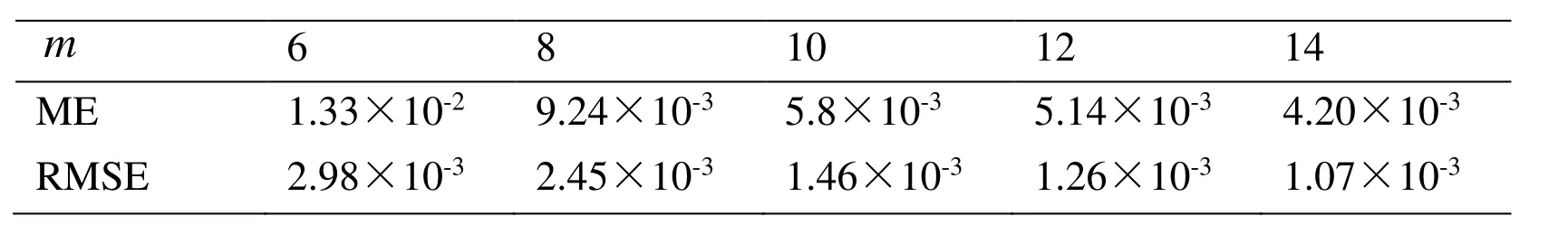
Table 1: For the non-harmonic boundary value problem of the Laplace equation,comparing the accuracy with different values of

In above, it can be seen that the number of collocation pointsused in the MSDTM is in general much larger than the number of unknown coefficientsis the number of the Trefftz bases used in the numerical solution, it cannot be too large to avoid the highly ill-conditioned behavior of the resultant linear system. On the other hand, in order to match the given boundary conditions accurately, we impose more collocation points to generate more linear equations. Due to these reasons the linear system is usually highly over-determined.

4.2 Inverse Cauchy problems

Before embarking the numerical tests of the presented method to solve the inverse Cauchy problems, we concern with the stability of the MSPM and the MSDTM, in the case when the boundary data are contaminated by the random noise. Thus we investigate the numerical results by adding a different level of random noise on the boundary data:

Example 5.In this example we consider an inverse Cauchy problem of Poisson equation as following:

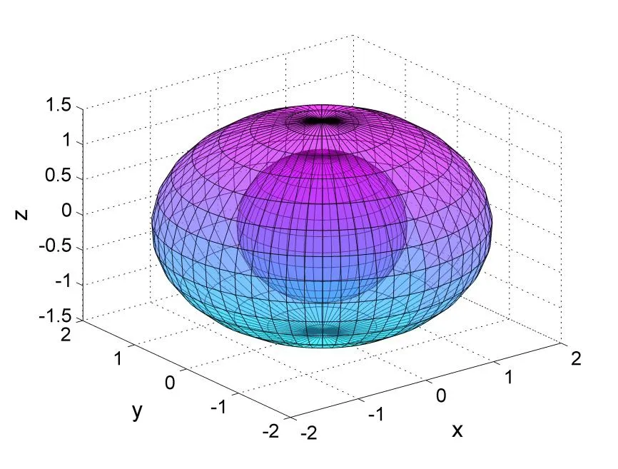
Figure 5: An ellipsoidal vessel with non-uniform thickness, domain for example 5

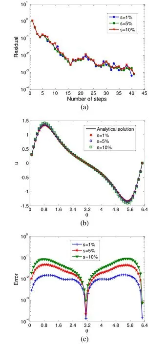
Figure 6: For example, 5 of a 3D Poisson problem in an irregular domain, (a) the convergence rate, (b) the comparison of the numerical and exact solutions, and (c) the numerical error

In Tab. 2 we list the ME and the RMSE ofat totally 8000 points infor different,but other parameters are fixed to be. It can be seen that the MSDTM is convergent fast and then situates.

Table 2: For example 5 comparing the accuracy with different values of

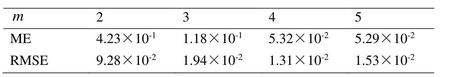
Table 2: For example 5 comparing the accuracy with different values of

Example 6.In this example we consider the following inverse Cauchy problem of Poisson equation:

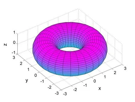
Figure 7: A torus centered at origin, domain for example 6

Fig. 9 lists the analytical solution and numerical solutions for u on lower half portion of the torus with 10% level of data noise. Even for a relatively high amount of noise 10%added into the data, the numerical results still agree quite well with the analytical solution,indicating that the MSPM and the MSDTM yields accurate and stable numerical results for noisy data.

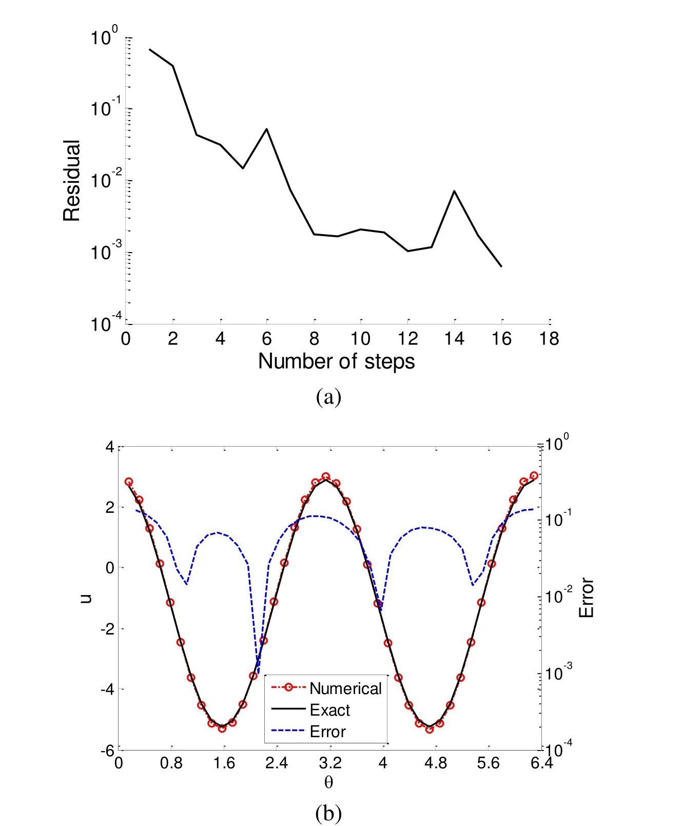
Figure 8: For example, 6 of a 3D Poisson problem in a torus domain, (a) the convergence rate, (b) the comparison of the numerical and exact solutions. The error reads with respect to the right axis

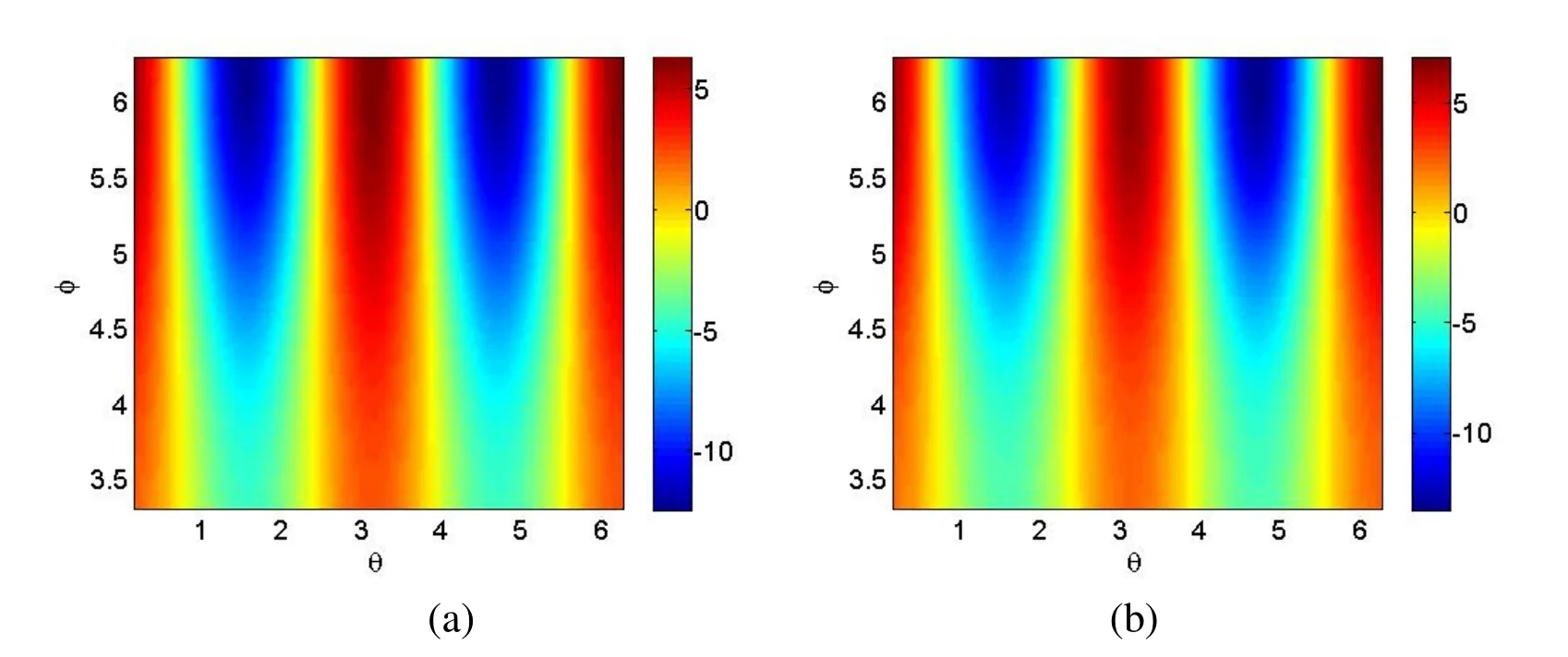
Figure 9: Distributions of (a) the analytical solutions and (b) the numerical solutions for u on the under-specified surface obtained using the MSPM and the MSDTM with s=10%

Example 7. We consider the following inverse Cauchy problem of the Poisson equation:

The Dirichlet and Neumann boundary conditions are over-specified via

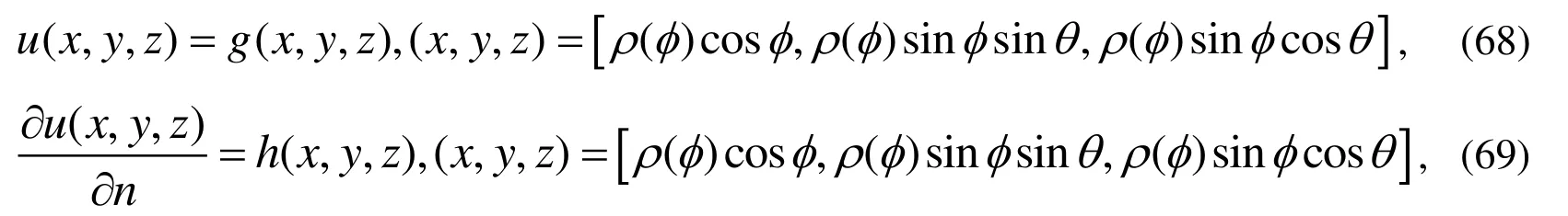
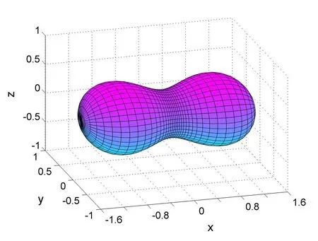
Figure 10: A peanut-shaped domain, domain for example 7

Fig. 12(a) gives the distribution of the analytical solution for u on the under-specified surface. Figs. 12(b-d) show the distributions of the numerical solutions on the underspecified surface obtained by using the MSPM and the MSDTM withandnoisy Cauchy data, respectively. As shown in these figures, the numerical results under different noise level are in good agreement with the analytical solution. Furthermore,the numerical solutions converge to the corresponding analytical solutions as the amount of noise decreases. This clearly shows the computational efficiency and accuracy of the proposed numerical scheme. On the other hand, Figs. 13(a-d) display the error surfaces of the numerical results on the under-specified surface, with exact input data, 1% noisy Cauchy data, 5% noisy Cauchy data, and 10% noisy Cauchy data, respectively. It can be seen that, even for a relatively high amount of noise level (10%), the numerical results remain accurate and stable, and converge to the corresponding analytical solution as noise level decreases.

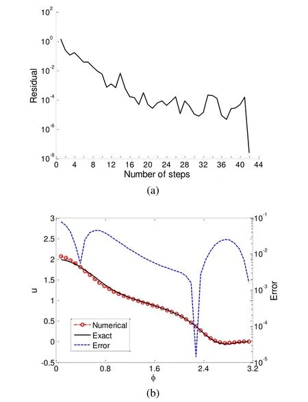
Figure 11: For example 7 of a 3D Poisson problem in a peanut-shaped domain, (a) the convergence rate of MSDTM, (b) comparing numerical and exact solutions and numerical error. The error reads with respect to the right axis

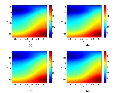
Figure 12: Distribution of (a) the analytical solutions and distributions of the numerical solutions for u on the under-specified surface obtained using the MSPM and the MSDTM with (b) s=1%, (c) s=5% and (d) s=10% noisy Cauchy data

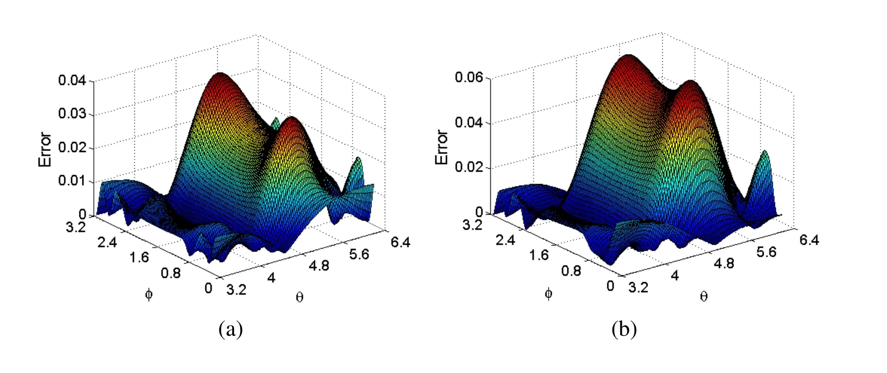
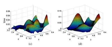
Figure 13: Error surfaces of u on the under-specified surface obtained using the MSDTM with (a) s=0, (b) s=1%, (c) s=5% and (d) s=10% noisy Cauchy data

Example 8.In this example we consider an inverse Cauchy problem of the Laplace equation in a central hollow sphere [Wang, Chen, Qu et al. (2016)]. The inner and outer radii of the spherical shell are 1 and 2, respectively. The Dirichlet and Neumann boundary conditions are over-specified on the outer surface. The analytical solution is

It should be noted that the MSPM is not needed due to the absence of the nonhomogeneous term. To compare with the boundary element method (BEM), Fig. 14 displays the relative error surfaces of the numerical results for the flux on the inner boundary, with exact input data, 1%, 3%, and 5% noisy Cauchy data, respectively. We take, and. Comparing with Fig. 4 in Wang et al. [Wang,Chen, Qu et al. (2016)], our numerical results are slightly accurate for the various noise level. Furthermore, the proposed method is simpler and faster to implement than the boundary element methods since the MSDTM does not require the time-consuming numerical integrations.

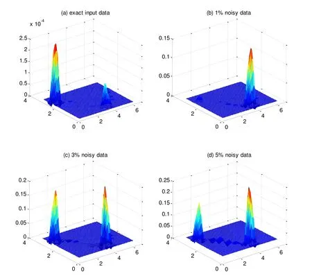
Figure 14: Relative error surfaces of the fluxes on the inner boundary obtained using the MSDTM with (a) exact input data, (b) 1%, (c) 3% and (d) 5% noisy data

Example 9.As the last example we consider an inverse Cauchy problem of the Laplace equation in a torus [Wang, Chen, Qu et al. (2016)], prescribed by the following parametric equation:

In this 3D case, the accessible part of the boundary is specified as

To compare with the boundary element method, Tab. 3 lists the MEs and CPU times of the numerical results on the under-specified surface obtained by using the BEM and the MSDTM with various noisy Cauchy data. In the calculation, the BEM used 48 torus exact elements is in conjunction with the TSVD-GCV regularization technique. In the MSDTM we take, and. It can be seen from Tab. 3 that the MSDTM is more accurate than the BEM for various noise levels. On the other hand, the BEM requires high amount of CPU time because of expensive numerical integration and regularization.

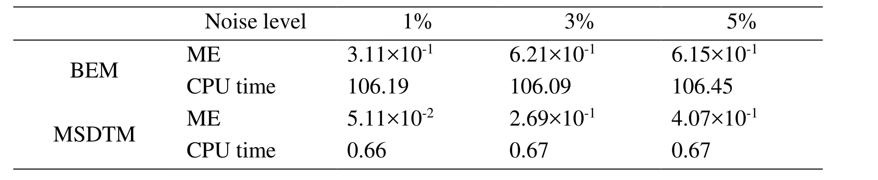
Table 3: For example 9 comparing the MEs and CPU time by using the BEM and the MSDTM with various noise levels

5 Conclusions

A simple multiple/scale polynomial method (MSPM) and multiple/scale/direction Trefftz method (MSDTM) were developed for the Poisson equation in an arbitrary threedimensional (3D) domain. The scales and directions are fully determined by the collocation points and the planar orientations. The proposed method is truly mesh-free and integrationfree and its equation system has a small number of unknown coefficients. By using a simple multiple-scale post-conditioner and a simple three-dimensional Trefftz basis, the method can reduce the ill-condition of the resultant linear system. The numerical results demonstrated that the MSPM and the MSDTM is very efficient, even for that adding a large random noise up to 10%.

Acknowledgement: The work described in this paper was supported by the Thousand Talents Plan of China (Grant No. A1211010), the Fundamental Research Funds for the Central Universities (Grant nos. 2017B656X14, 2017B05714), the Postgraduate Research& Practice Innovation Program of Jiangsu Province (Grant No. KYCX17_0487), and the Natural Science Foundation of Shandong Province of China (Grant No. ZR2017BA003).

Reference

Algahtani, H. J.(2006): A meshless method for non-linear Poisson problems with high gradients. Computer Assisted Mechanics and Engineering Sciences, vol. 13, no. 3, pp. 367.

Atluri, S. N.; Kim, H. G.; Cho, J.(1999): A critical assessment of the truly meshless local petrov-galerkin (mlpg), and local boundary integral equation (lbie) methods. Computational mechanics, vol. 24, no. 5, pp. 348-372.

Atluri, S. N.; Zhu, T.(1998): A new meshless local Petrov-Galerkin (mlpg) approach in computational mechanics. Computational mechanics, vol. 22, no. 2, pp. 117-127.

Chapko, R.; Johansson, B. T.(2012): A direct integral equation method for a Cauchy problem for the Laplace equation in 3-dimensional semi-infinite domains. Computer Modeling in Engineering & Sciences, vol. 85, pp. 105-128.

Chen, C.; Fan, C.; Wen, P.(2012): The method of approximate particular solutions for solving certain partial differential equations. Numerical Methods for Partial Differential Equations, vol. 28, no. 2, pp. 506-522.

Chen, Y. W.; Yeih, W. C.; Liu, C. S.; Chang, J. R.(2012): Numerical simulation of the two-dimensional sloshing problem using a multi-scaling Trefftz method. Engineering Analysis with Boundary Elements, vol. 36, no. 1, pp. 9-29.

Cheng, A.; Golberg, M.; Kansa, E.; Zammito, G.(2003): Exponential convergence and hc multiquadric collocation method for partial differential equations. Numerical Methods for Partial Differential Equations, vol. 19, no. 5, pp. 571-594.

Cheng, A. D.(2000): Particular solutions of Laplacian, Helmholtz-type, and polyharmonic operators involving higher order radial basis functions. Engineering Analysis with Boundary Elements, vol. 24, no. 7, pp. 531-538.

Cho, H. A.; Golberg, M.; Muleshkov, A.; Li, X.(2004): Trefftz methods for time dependent partial differential equations. Computers, Materials & Continua, vol. 1, pp. 1-38.

Fan, C. M.; Li, P. W.; Yeih, W.(2015): Generalized finite difference method for solving two-dimensional inverse Cauchy problems. Inverse Problems in Science and Engineering,vol. 23, no. 5, pp. 737-759.

Golberg, M.; Muleshkov, A.; Chen, C.; Cheng, A. D.(2003): Polynomial particular solutions for certain partial differential operators. Numerical Methods for Partial Differential Equations, vol. 19, no. 1, pp. 112-133.

Golberg, M. A.(1995): The method of fundamental solutions for Poisson’s equation.Engineering Analysis with Boundary Elements, vol. 16, no. 3, pp. 205-213.

Hu, H.; Chen, J.(2008): Radial basis collocation method and quasi-Newton iteration for nonlinear elliptic problems. Numerical Methods for Partial Differential Equations, vol. 24,no. 3, pp. 991-1017.

Hu, H. Y.; Li, Z. C.; Cheng, A. H. D.(2005): Radial basis collocation methods for elliptic boundary value problems. Computers & Mathematics with Applications, vol. 50, no. 1, pp.289-320.

Jin, B.(2004): A meshless method for the Laplace and biharmonic equations subjected to noisy boundary data. Computer Modeling in Engineering & Sciences, vol. 6, pp. 253-262.

Kansa, E. J.(1990): Multiquadrics-A scattered data approximation scheme with applications to computational fluid-dynamics-I surface approximations and partial derivative estimates.Computers & Mathematics with Applications, vol. 19, no. 8, pp. 127-145.

Ku, C. Y.; Kuo, C. L.; Fan, C. M.; Liu, C. S.; Guan, P. C.(2015): Numerical solution of three-dimensional Laplacian problems using the multiple scale Trefftz method.Engineering Analysis with Boundary Elements, vol. 50, pp. 157-168.

Lamichhane, A.; Chen, C.(2015): The closed-form particular solutions for Laplace and biharmonic operators using a Gaussian function. Applied Mathematics Letters, vol. 46, pp.50-56.

Li, Z. C.; Lu, T. T.; Hu, H. Y.; Cheng, A. H.(2008): Trefftz and collocation methods.WIT press.

Li, Z. C.; Lu, T. T.; Huang, H. T.; Cheng, A. H. D.(2007): Trefftz, collocation, and other boundary methods-a comparison. Numerical Methods for Partial Differential Equations, vol. 23, no. 1, pp. 93-144.

Libre, N. A.; Emdadi, A.; Kansa, E. J.; Rahimian, M.; Shekarchi, M.(2008): A stabilized RBF collocation scheme for Neumann type boundary value problems. Computer Modeling in Engineering & Sciences, vol. 24, no. 1, pp. 61-80.

Liu, C. S.(2007): A modified Trefftz method for two-dimensional Laplace equation considering the domain’s characteristic length. Computer Modeling in Engineering &Sciences, vol. 21, no. 1, pp. 53-65.

Liu, C. S.(2008a): A modified collocation Trefftz method for the inverse Cauchy problem of Laplace equation. Engineering Analysis with Boundary Elements, vol. 32, no. 9, pp. 778-785.

Liu, C. S.(2008b): A highly accurate MCTM for inverse Cauchy problems of Laplace equation in arbitrary plane domains. Computer Modeling in Engineering & Sciences, vol.35, no. 2, pp. 91-111.

Liu, C. S.(2012a): An equilibrated method of fundamental solutions to choose the best source points for the Laplace equation. Engineering Analysis with Boundary Elements, vol.36, no. 8, pp. 1235-1245.

Liu, C. S.(2012b): Optimally generalized regularization methods for solving linear inverse problems. Computers, Materials & Continua, vol. 29, no. 2, pp. 103-127.

Liu, C. S.(2013): A two-side equilibration method to reduce the condition number of an ill-posed linear system. Computer Modeling in Engineering & Sciences, vol. 91, pp. 17-42.

Liu, C. S.(2016): A simple Trefftz method for solving the Cauchy problems of threedimensional Helmholtz equation. Engineering Analysis with Boundary Elements, vol. 63,pp. 105-113.

Liu, C. S.; Atluri, S. N.(2013): Numerical solution of the Laplacian Cauchy problem by using a better postconditioning collocation Trefftz method. Engineering Analysis with Boundary Elements, vol. 37, no. 1, pp. 74-83.

Liu, C. S.; Qu, W.; Chen, W.; Lin, J.(2017): A novel Trefftz method of the inverse Cauchy problem for 3D modified Helmholtz equation. Inverse Problems in Science and Engineering, vol. 25, no. 9, pp. 1278-1298.

Liu, C. S.; Yeih, W.; Atluri, S. N.(2009): On solving the ill-conditioned system Ax=b:general-purpose conditioners obtained from the boundary-collocation solution of the Laplace equation, using Trefftz expansions with multiple length scales. Computer Modeling in Engineering & Sciences, vol. 44, no. 3, pp. 281-311.

Lv, H.; Hao, F.; Wang, Y.; Chen, C. S.(2017): The MFS versus the Trefftz method for the Laplace equation in 3d. Engineering Analysis with Boundary Elements, vol. 83, no. 1,pp. 133-140.

Pradhan, D.; Shalini, B.; Nataraj, N.; Pani, A. K.(2011): A Robin-type nonoverlapping domain decomposition procedure for second order elliptic problems. Advances in Computational Mathematics, vol. 34, no. 4, pp. 339-368.

Qu, W.; Chen, W.; Fu, Z.(2015): Solutions of 2d and 3d non-homogeneous potential problems by using a boundary element-collocation method. Engineering Analysis with Boundary Elements, vol. 60, no. 1, pp. 2-9.

Shen, S. N. A. S.(2002): The meshless local Petrov-Galerkin (mlpg) method: a simple &less-costly alternative to the finite element and boundary element methods. Computer Modeling in Engineering & Sciences, vol. 3, no. 1, pp. 11-51.

Tian, H. Y.; Reutskiy, S.; Chen, C.(2008): A basis function for approximation and the solutions of partial differential equations. Numerical Methods for Partial Differential Equations, vol. 24, no. 3, pp. 1018-1036.

Tsai, C.; Cheng, A. D.; Chen, C.(2009): Particular solutions of splines and monomials for polyharmonic and products of Helmholtz operators. Engineering Analysis with Boundary Elements, vol. 33, no. 4, pp. 514-521.

Wang, F.; Chen, W.; Qu, W.; Gu, Y.(2016): A BEM formulation in conjunction with parametric equation approach for three-dimensional Cauchy problems of steady heat conduction. Engineering Analysis with Boundary Elements, vol. 63, no. 1, pp. 1-14.

Wei, T.; Hon, Y.; Cheng, J.(2003): Computation for multidimensional Cauchy problem.SIAM Journal on Control and Optimization, vol. 42, no. 2, pp. 381-396.

Zhu, T.; Zhang, J.; Atluri, S.(1999): A meshless numerical method based on the local boundary integral equation (lbie) to solve linear and non-linear boundary value problems.Engineering Analysis with Boundary Elements, vol. 23, no. 5, pp. 375-389.