Attractors for a Caginalp Phase-field Model with Singular Potential

Alain Miranvilleand Charbel Wehbe

1 Laboratoire de Math´ematiques et Applications,UMR CNRS 7348,SP2MI,Boulevard Marie et Pierre Curie-T´el´eport 2,F-86962 Chasseneuil Futuroscope Cedex,France.

2 Xiamen University,School of Mathematical Sciences,Xiamen,Fujian,P.R.China.

Abstract.We consider a phase field model based on a generalization of the Maxwell Cattaneo heat conduction law,with a logarithmic nonlinearity,associated with Neumann boundary conditions.The originality here,compared with previous works,is that we obtain global in time and dissipative estimates,so that,in particular,we prove,in one and two space dimensions,the existence of a unique solution which is strictly separated from the singularities of the nonlinear term,as well as the existence of the finite-dimensional global attractor and of exponential attractors.In three space dimensions,we prove the existence of a solution.

Key words: Caginalp phase-field system,Maxwell-Cattaneo law,logarithmic potential,Neumann boundary conditions,well-posedness,global attractor,exponential attractor.

1 Introduction

The Caginalp phase-field model

has been proposed to model phase transition phenomena,for example melting-solidification phenomena,in certain classes of materials.Caginalp considered the Ginzburg-Landau free energy and the classical Fourier law to derive his system,see,e.g.,[1,2].Here,u denotes the order parameter and θ the(relative)temperature.Furthermore,all physical constants have been set equal to one.For more details and references we refer the reader to[2-4]. This model has been extensively studied(see,e.g.,[5]and the references therein). Now,a drawback of the Fourier law is the so-called”paradox of heat conduction”,namely,it predicts that thermal signals propagate with infinite speed,which,in particular,violates causality(see,e.g.,[5]).One possible modification,in order to correct this unrealistic feature,is the Maxwell-Cattaneo law. We refer the reader to[3,5,6]for more discussions on the subject.

In this paper,we consider the following model

which is a generalization of the original Caginalp system(see[2]).In this context α is the thermal displacement variable,defined by

As mentioned above the Caginalp system can be obtained by considering the Ginzburg-Landau free energy

the enthalpy H=u+θ and by writing

where d ＞0 is a relaxation parameter,∂udenotes a variational derivative and q is the thermal flux vector.Setting d=1 and taking the usual Fourier law

we find(1.1)-(1.2).

The Maxwell-Cattaneo law reads

where η is a relaxation parameter;when η=0,one recovers the Fourier law.Taking for simplicity η=1,it follows from(1.8)that

hence the following second-order(in time)equation for the relative temperature

Integrating finally(1.11)between 0 and t,we obtain the equation

where f depends on the initial data(for u and θ),which reduces to(1.4)when f vanishes.Furthermore,noting that,(1.1)can be rewritten in the equivalent form(1.3).

We endow this model with Neumann boundary conditions and initial conditions.Then,we are led to the following initial and boundary value problem(P):

in a bounded and regular domain Ω⊂Rn(n is to be specified later),with boundary ∂Ω.

We assume here that g=G′,where

i.e.,

In particular,it follows from(1.18)that

Concerning the mathematical setting,we introduce the following Hilbert spaces

Our aim in this paper is to prove the existence of a solution in the case of the logarithmic nonlinearity(1.18).The main difficulty is to prove that the order parameter is separated from the singularities of g.In particular,we are only able to prove such a property in one and two space dimensions.In three space dimensions,we prove the existence of a solution.

Throughout the paper,the same letter c(and,sometimes,c′)denotes constants which may change from line to line.

2 A priori estimates

The singularities of the potential g lead us to define the quantity

We set

We rewrite(1.13)in the form

We then rewrite(1.14)in the form

where

Integrating(2.3)over Ω,we obtain

In particular,we deduce from(2.4)that

hence

Furthermore,if〈H(0)〉=0,i.e.,〈u0+α1〉=0,we have conservation of the enthalpy,

Setting φ=φ-〈φ〉,we then have

We first sum(2.9)and δ1×(2.10)to have

where δ1＞0 is small enough so that,in particular,

and then sum(2.2)and δ2×(2.11),where δ2＞0 is small enough,to obtain

where

We now multiply(1.13)by-Δu,and have,owing to(1.19),

Summing(2.13)and δ3×(2.15),where δ3＞0 is small enough,we finally obtain

where

satisfies

We differentiate(1.13)with respect to time to find,owing to(1.14),

Finally,we multiply(1.14)by-Δα and we integrate over Ω to have

which implies

We sum(2.21)and δ4×(2.22),where δ4＞0 is small enough,to get

We then have

where

Now we sum(2.20)and δ5×(2.24),where δ5＞0 is small enough,to get

where

Finally,we sum(2.16)and δ6×(2.26),where δ6＞0 is small enough,to get

where

satisfies

Using(2.16),(2.20)and Gronwall’s lemma,we deduce

and

Note that

Using(2.31)and(2.33),we deduce from(2.32)the following inequality

We rewrite(1.13)in an elliptic form for t≥0 fixed,

We multiply(2.35)by-Δu.Using(1.19),H¨older and Young’s inequalities,we obtain

Using now(2.31),(2.34)and(2.37)we find

Applying Gronwall’s lemma to(2.28)and using(2.30)we have

By(2.34),(2.38)and(2.39)we get

Our aim now is to prove that u a priori satisfies

where δ＞0 is to be specified later.

In one space dimension,we have,owing to the embeddingan estimate onin L∞(R+×Ω).It is then not difficult to prove the separation property(2.41)for solutions to the parabolic equation

with right-hand side h∈L∞(R+×Ω).

Indeed,by(2.40),h satisfies

We prove(see[16]and[20]):

Thus,due to the comparison principle,we deduce the following inequalities:

Estimates(2.43)-(2.46)imply that

Combining(2.40)and(2.47),we obtain

In particular

We now turn to thetwo-dimensional case.To this end,we derive further a priori estimates.

We then multiply(1.14)by Δ2α to get

Summing(2.50)and ϵ×(2.51),where ϵ＞0 is small enough such that 1-2ϵ＞0 and 1-ϵ＞0,we have

where

and

Applying Gronwall’s lemma to(2.52),we have

Furthermore,by(2.40)we get

Now,we differentiate(1.13)with respect to time to have,owing to(1.14),

where

We apply Gronwall’s lemma to(2.58),to have

Hence we have to estimate the termds.To do so,we first prove the following lemma.

Lemma 2.1.∀M＞0:

where c′only depends on M.

Proof.We can assume,without loss of generality,that

We fix M＞0 and multiply(2.42)by g(u)eM|g(u)|to have:

In order to estimate the second term in the right-hand side of(2.63),we use the following Young’s inequality

where

Taking a=N|h|and b=N-1|g(u)|eM|g(u)|,where N＞0 is to be fixed later,in(2.64),we obtain

Now,if|g(u)|≤1,then

Furthermore,if|g(u)|≥1,then|g(u)|eM|g(u)|≥1 and

where c only depends on M.We thus deduce from(2.63)and(2.66)the following inequality

where c′only depends on M.

To conclude,we use the following Orlicz’s embedding inequality

where c only depends on Ω and N.It then follows from(2.43),(2.67)and(2.68)that

Noting finally that

where c only depends on M,(2.69)yields the desired inequality(2.60).

It is not difficult to show,by comparing growths,that the logarithmic function g satisfies

Therefore,

whence,owing to(2.60),

Thus φ in(2.57)satisfies,owing to(2.60)(for p=4)and the above a priori estimates(which imply thatΩ)),

hence,

Furthemore,we have

Using(2.75)and(2.76)in(2.59)and by(2.48),we deduce

By(2.48),(2.53),(2.55)and(2.77),we deduce from(2.54)

Rewriting again(1.13)in the form

we have,owing to the above estimates,

and the separation property follows as in the one-dimensional case.

3 Existence of solutions

We have the

Theorem 3.1.(i)In one space dimension,we assume that

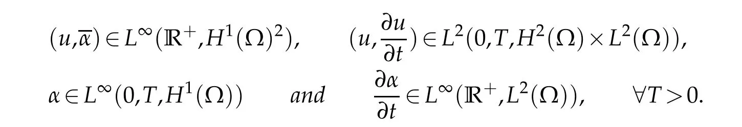
Then,(1.13)-(1.16)possesses a unique solution(u,α,)such that

(ii)In two space dimension,we assume that

Then,(1.13)-(1.16)possesses a unique solution(u,α,)such that

(iii)In three space dimension,we consider the set K={φ ∈L2(Ω),-1 ≤φ ≤1, a.e.in Ω}and we assume that(u0,α0,α1)∈FK=(K∩H1(Ω))×H1(Ω)×L2(Ω).Then,(1.13)-(1.16)possesses a unique solution(u,α,)such that

Moreover for all t＞0,‖u(t)‖L∞(Ω)≤1 and the set{x∈Ω/|u(x,t)|=1}has measure zero.Proof.In one and two space dimensions,the proof of existence is standard,once we have the separation property(2.41),since the problem then reduces to one with a regular nonlinearity.Indeed,we consider the same problem,in which the logarithmic function g is replaced by the C1function

where δ is the same constant as in(2.41).

This function meets all the requirements of[25]to have the existence of a regular solutionFurthermore,It is not difficult to see that g and gδsatisfy(1.19),(1.20)and(2.71),for the same constants.We can thus derive the same estimates as above,with the very same constants.

Since g and gδcoincide on[-δ,δ],we finally deduce that uδis solution to the original problem.

In three space dimension,following an idea of Debussche and Dettori[7]we consider the approximation of the function g by a polynomial of odd degree gN,and the boundary value problem(PN)that one obtains by replacing g by gNin problem(P)

The existence and uniqueness of a solutionto problem(3.5)-(3.8)have been proved in[25].We then construct the solution of problem(1.13)-(1.16)as the limit ofas N →+∞.Indeed,we first derive uniform estimates with respect to N for problem(3.5)-(3.8).Replacing(u,α)in(2.16)by(uN,αN),we write

where

satisfies

Using Gronwall’s Lemma we have

where c is independent of N.Hence there exists a subsequence ofthat we denote again bywhich satisfies as N →+∞

Moreover,integrating(3.9)over(0,t),we obtain

where c is independent of N.We then deduce

Replacing H by HNin(2.5),we write

which can be written as

Integrating(3.20)over(0,t)we obtain

We then deduce

Using the equivalent norm in H1(Ω)we get

where c is independent of N.We deduce that

We now multiply(3.5)by gN(uN)and integrate over Ω using≥-c to have

Integrating(3.25)over(0,t),we deduce

where c is independent of N and Q=Ω×(0,T).

By(3.26)and for a subsequence we obtain

Letting N →+∞in the equation(3.5),we deduce from(3.15),(3.17),(3.18)and(3.27)thatsatisfies

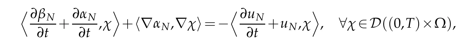
where〈.,.〉denote the duality product between D′((0,T)×Ω)and D((0,T)×Ω).

Then letting N-→+∞,using(3.13),(3.15),(3.17)and(3.24)we deduce

Moreover using[12],(3.13),(3.17)on the one hand and(3.15),(3.24)on the other hand implies that as N-→+∞

so that in particular u(x,0)=u0and α(x,0)=α0in Ω.

Furthermore we deduce from(3.15)thatOn the other hand we haveso that

Using Strauss Theorem,we getand there exist a subsequencesuch that in particular asµ→+∞we have

Note also that using Lions’Theorem and(3.13)-(3.15),(3.17)and(3.24),we get

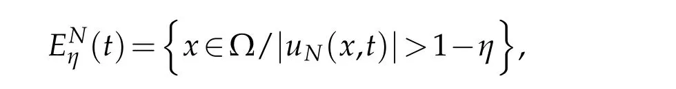
We now prove that g⋆=g(u)and the set{x ∈Ω,|u(x,t)|=1}has measure zero.To do so we adapt a method introduced by Debussche and Dettori[7].For an arbitrary small η ∈(0,1)and for all t∈(0,T),we set

Integrating(3.9)over(t,t+r),we obtain

To continue the proof of the theorem we state the following two lemmas.

Lemma 3.1.There exists a constant c such that for all r＞0

Proof.Replacing(u,α)in(2.20)by(uN,αN),we write

Applying the uniform Gronwall’s Lemma to(3.38),using(3.11)and(3.36)we deduce that∀s＞0,

which completes the proof of(3.37).

Lemma 3.2.There exists a constant c such that for all r＞0

Proof.Applying Gronwall’s lemma to(3.9),using(3.11)we deduce that

By(3.37)and(3.41),we get from(3.25)the inequality(3.40).

Using Lemma 3.2 we deduce that

and thus

which implies that

Thus letting N →+∞we deduce from(3.30),(3.43)and Fatou’s Lemma that

where|Eη(t)|and χη(t)respectively stand for the measure of the set{x ∈Ω,|u(x,t)|＞1-η}and for its characteristic function.Letting then η→0,it follows that for all t∈(0,T)

It follows respectively from(3.30)and(3.44)that for all t∈(0,T)and almost every x∈Ω

Then using Lions([8],lemma 1.3,p.12)it follows from(3.26)and(3.45)that

so that g∗=g(u).

We then have

which is equivalent to

In one space dimension,by(2.41)we have for all t≥0,

We set δ0=min(δ1,δ2)and then deduce

hence

Remark 3.1.In two space dimension,we have

where

This yields,owing to Gronwall’s lemma,

Integrating then(3.52)over Ω,we have,as above,

Noting that it follows from(3.58)that

where c depends on T and δ0,which yields,in particular,

we finally deduce from(3.60)-(3.62)that

where c depends on T and δ0,hence the uniqueness,as well as the continuous dependence with respect to the initial data.

Thanks to Theorem 3.1(i),we can define the dissipative semigroupassociated with problem(1.13)-(1.16)on the phase space

Indeed,by(3.2)we have

Concerning the two-dimensional case,we have that

is a bounded absorbing set for S(t)in Ψ0.Indeed,we have

4 Global attractor

We have the

Theorem 4.1.(i)If n=1,we take the initial conditions inThen the semigroup(t),t≥0,defined fromto itself possesses the connected global attractorin

(ii)If n=2,the initial conditions belong to.Then(t)defined fromto itself possesses the connected global attractor

Proof.We use a semigroup decomposition argument(see,e.g.,[6])consisting in splitting the semigroupt≥0,into the sum of two families of operators:where operatorsgo to zero as t tends to infinity while operatorsare compact.

This corresponds to the following solution decomposition

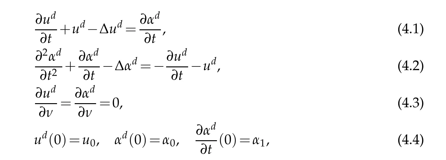
where f(s)=g(s)-s(f and g satisfy the same properties)and with initial data belonging toMultiplying(4.1)by(4.2)byand summing the resulting equations,we have

we get

where ϵ3＞0 is small enough,and we have in particular

Summing(4.9)and ϵ4×(4.11)where ϵ4＞0 is small enough,we have

where

Applying Gronwall’s lemma to(4.13),we write

Considering equation(4.10)and repeating exactly the estimates that gave(2.13),we get

where

and ϵ5＞0 and ϵ6＞0 are small enough so that we have in particular

Applying Gronwall’s lemma to(4.17),we have

Combining(4.15)and(4.20),we obtain

Now,we consider system(4.5)-(4.8).

We multiply(4.5)by-Δuc.Integrating over Ω we have

Summing the resulting equations,we get

Summing(4.25),(4.26)and ϵ7×(4.27)where ϵ7＞0 is small enough,we have

where

By(3.2),we deduce that

By(4.30),we deduce from(4.28)the following estimate

Applying Gronwall’s lemma to(4.31)(noting that ψ1(0)=0)and by using(4.29)we obtain

Summing now(4.23),(4.33)and ϵ8×(4.24),where ϵ8＞0 is small enough,we deduce that

where

Applying Gronwall’s lemma to(4.34),using(3.2)and(4.35)we have

Combining(4.32)and(4.36),we get

Hence,the operator S2(t)is asymptotically compact in the sense of the Kuratowski measure of noncompactness(see[18]),which concludes the existence part of Theorem 4.1(i).

In order to prove part(ii)of Theorem 4.1,we now take the initial data inthen multiply(4.1)byand(4.2)bySumming the two resulting equations,we end up with

We multiply(4.10)by Δ2αd.Integrating over Ω,and using∀φ ∈H3(Ω),c＞0,we have

Summing(4.39)and ϵ9×(4.40)where ϵ9＞0 is small enough,we deduce that

and we have,in particular,

Summing then(4.38)and ϵ10×(4.41),where ϵ10＞0 is small enough,we obtain

where

Applying Gronwall’s lemma to(4.43),using(4.42)and(4.44)we get

By(4.21)and the continuous injection F2⊂F1,we have

We then deduce from(4.45)and(4.46)the following estimate

Concerning system(4.5)-(4.8),we multiply(4.5)by Δ2uc.Integrating over Ω,we get

Summing(4.26),(4.27)and(4.48)we obtain

Summing(4.49),(4.50)and ϵ11×(4.51)where ϵ11＞0 is small enough,we obtain

where

Furthermore,we have

Inserting(4.54)and(4.55)in(4.52)and applying Gronwall’s lemma to the resulting estimate,we deduce by(4.53)that

Combining(4.37)and(4.56)we have

which completes the proof of the theorem.

We define for what follows the following invariant sets:in one space dimension,=whereis the bounded absorbing set forinand in two space dimensions,whereis the bounded absorbing set forinIn what follows,we will work in these two subspacesandwhich are positively invariant for

Now that the existence of the global attractor is proven,one natural question is to know whether this attractor has finite dimension in terms of the fractal or Hausdorff dimension.This is the aim of the final section.

5 Exponential attractors

The aim of this section is to prove the existence of exponential attractors for the semigroup S(t),t ≥0,associated to problem(1.13)-(1.16)in one and two space dimensions using the separation property(2.41).To do so,we need the semigroup to be Lipschitz continuous and satisfy the smoothing property,but also to verify a H¨older condition in time(see[18],[19],[28-30]).This is enough to conclude on the existence of exponential attractors,but before going further,let us recall the definition of an exponential attractor which is also called inertial set.

Definition 5.1.A compact set M is called an exponential attractor for({S(t)}t≥0,X),if

(i)A⊂M⊂X,where A is the global attractor,

(ii)M is positively invariant for S(t),i.e.S(t)M⊂M for every t≥0,

(iii)M has finite fractal dimension,

(iv)M attracts exponentially the bounded subsets of X in the following sense:∀B⊂X bounded, dist(S(t)B,M)≤Q(‖B‖X)exp(-αt), t≥0,

where the positive constant α and the monotonic function Q are independent of B,and dist stands for the Hausdorff semi-distance between sets in X,defined by

We start by stating an abstract result that will be useful in what follows(see[18]).

Theorem 5.1.Let Ψ and Ψ1be two Banach spaces such that Ψ1is compactly embedded into Ψ and S(t):Y-→Y be a semigroup acting on a closed subset Y of Ψ.We assume that

(i)

where

d is continuous,t≥0,d(t)→0 as t→+∞,and

Then S(t)possesses an exponential attractor M on Y.

In order to get the existence of exponential attractors in our case,we will use Theorem 5.1.We have the following result

Theorem 5.2.(i)In one space dimension,the semigroupcorresponding to equations(1.13)-(1.16)defined fromto itself satisfies a decomposition as in Theorem 5.1.

and

respectively.We start with the proof of(i).In that case the initial conditions belong toRepeating for(5.6)-(5.9)the estimates which led to(4.13)and(4.17),we then write(noting that

where

where

Here ϵ＞0 and δ＞0 are small enough so that we have in particular

An application of Gronwall’s lemma to(5.14)and(5.16)respectively yields

Combining(5.20)and(5.21),we get

Noting that

due to the continuous embedding H2(Ω)⊂L∞(Ω),and by(3.2),we have

Thus,

Choosing ϵ＞0 small enough and using(5.24)and(5.26),we deduce from(5.23)the following inequality

Integrating(5.27)over(0,t),by(5.13)we have

H¨older’s inequality,(3.2)and(5.5)yield

Analogously,we have

Choosing ϵ＞0 small enough and recalling(5.30)and(5.31),we obtain

where

Integrating(3.61)over(0,t),we get

Integrating then(5.32)over(0,t)and using(5.34)we deduce that

hence(5.28)yields

H¨older’s inequality and(5.5)yield

where

In particular

Applying Gronwall’s lemma to(5.40)and using(5.39)we deduce that

Finally,multiplying(5.10)by υ+and(5.11)byand proceeding exactly as above we deduce that

Combining(5.36),(5.41)and(5.42),we obtain

where h(t)=c′ect,with c and c′depending onWe can see that h is continuous.

We now turn to the two-dimensional case,and prove part(ii)of Theorem 5.2.To do so we take here the initial data inRepeating for(5.6)-(5.9)the estimates which led to(4.43),we then write

where

and ϵ＞0 is small enough so that

In particular

An application of Gronwall’s lemma yields

Furthermore,by(5.22)and the continuous embedding F2⊂F1,we get

By(5.48)and(5.49)we have

Concerning problem(5.10)-(5.13),we multiply(5.10)byand(5.11)bySumming the resulting equations,we then obtain

Analogously to(5.26),we write

By(3.4)and the continuous embedding,we have

so that

Choosing ϵ ＞0 small enough and recalling(5.52)and(5.54),we deduce from(5.51)the estimate

Integrating(5.55)over(0,t)and by(5.13)we get

By(5.35),we have

As above we have

Choosing ϵ＞0 small enough and by recalling(5.59)and(5.60),we deduce from(5.58)the estimate

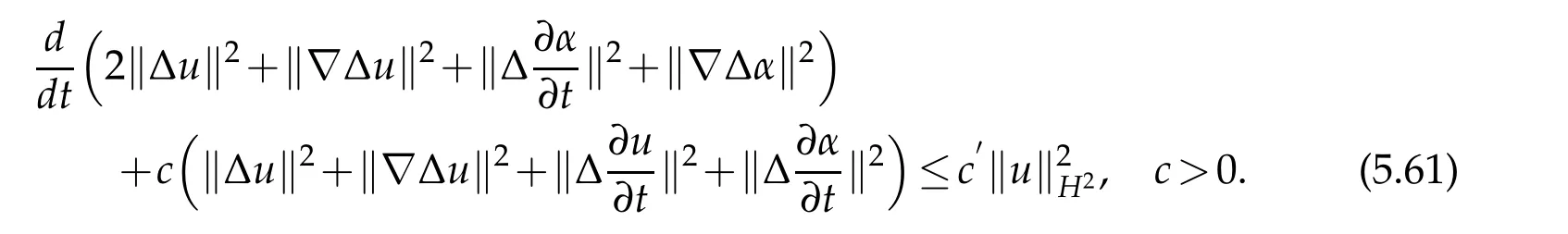
Integrating(5.61)over(0,t)and by(5.57)we have

Combining(5.57)and(5.62),we get

Inserting(5.63)in(5.56)we obtain

Noting that〈ξ〉=0,from(5.64)we deduce that

Combining(5.43)and(5.65),we obtain

which completes the proof.

Lemma 5.1.The semigroup S(t),t≥0 generated by the problem(1.13)-(1.16)is H¨older continuous on[0,T]×i=1,2(i depending on the space dimension).

Proof.We consider the one-dimensional case(the two-dimensional case can be treated similarly).The Lipschitz continuity in space is a consequence of(3.63).It just remains to prove the continuity in time(actually,a H¨older condition in time for the semigroup(t),t≥0).We assume that the initial data belong to.For every t1≥0 and t2≥0,owing to the above estimates,one gets:

where c depends on T.We multiply(1.14)byto obtain

Integrating(5.67)between t1and t2,we deduce from the above estimates that

We deduce from Theorem 5.2 and Lemma 5.1 the following result.

Theorem 5.3.The dynamical system(respectivelyassociated to(1.13)-(1.16)possesses,in one space dimension,an exponential attractorin(respectively,in two space dimensions,an exponential attractorin