A Novel Interacting Multiple-Model Method and Its Application to Moisture Content Prediction of ASP Flooding

1 Introduction

In practical applications, the industrial processes are always complex nonlinear dynamic systems, which are difficult and time-consuming to solve the mechanism models directly.With the development of computers, data-driven system identification can be viewed as an alternative way. Nonlinear system identification is to estimate models of nonlinear dynamic systems from observed input-output data, it is a subject with a long history of research interest and still remains active because of the need to accommodate more requirements and improve operating processes. Many traditional modeling methods are used in nonlinear system identification, such as nonlinear auto-regressive exogenous input (NARX) models [Hong, Tran and Yang (2010)], artificial neural network (ANN)models [Wang, Yan and Shi (2013)], support vector machine (SVM) models [Yan, Shao and Wang (2004)], Hammerstein models [Qi and Li (2008)], Wiener models [Qi and Li(2009)]. These methods have exposed several disadvantages in actual applications. Firstly,the prediction model often provide a scalar prediction only at any sampling point without any measure of the confidence in that prediction, because the models do not consider the uncertainty of model structure. A more suitable model should provide predictive error for each prediction, or even supply a complete predictive distribution. Secondly, overfitting problems often exist because much more attention is paid to reducing the errors at training points, especially in ANN models. GP models can be ideally suitable for solving the first problem. And RELM models can solve the second one. Moreover, model renewal caused by adding new meaningful samples can also help to alleviate the second problem.

GP models, also known as kriging in geostatistics, have developed rapidly in recent years because of the capability of providing the uncertainties of the predicted outputs and the relatively less number of optimizing parameters. O’Hagan et al. [O’Hagan and Kingman(1978)] first introduced the GP model approach to curve fitting. Later, Rasmussen[Rasmussen (1996)] compared GP models with other widely used models, leading to a rapidly growing attention to GP models. The paper by Rasmussen [Rasmussen (2006)]provided a long-needed, systematic and unified treatment of theoretical and practical aspects of GP models in machine learning. Ažman et al. [Ažman and Kocijan (2007)]used GP models for black-box modelling of Biosystems. A biomass concentration estimator for bath biotechnological processes by Bayesian GP regression is proposed di Sciascio et al. [di Sciascio and Amicarelli (2008)]. And Kocijan et al. [Kocijan and Likar(2008)] utilized GP models for gas-liquid separator modelling and simulation. Also, there are lots of variants about GP models, such as recursive GPR [Chan, Liu, Chen et al.(2013)], moving-window GPR [Ni, Tan, Ng et al. (2012)], sparse GP [Seeger, Williams,Lawrence et al. (2003); Csató and Opper (2002); Keerthi and Chu (2005)]. In general, GP models have been increasingly viewed as an alternative approach to other traditional modelling methods [Gregorčič and Lightbody (2008); Deisenroth, Zheng, Chen et al.(2009); Gregorčič and Lightbody (2009)].

Extreme learning machine (ELM) is a single-hidden layer feedforward neural network(SLFN) in fact, but unlike conventional one, ELM randomly chooses hidden nodes and analytically determines the output weights, leading to an extremely fast learning speed[Huang, Zhu and Siew (2006)]. Because of the good characteristics, ELM has been gradually used in nonlinear system identifications. A regression algorithm of quasi-linear model with ELM is proposed for nonlinear system identification [Li, Xie and Jin (2015);Li, Jia, Liu et al. (2014)] utilized OS-ELM for adaptive control of nonlinear discrete-time systems. A new method via ELM based Hammerstein model is proposed by Tang et al.[Tang, Li and Guan (2014)] for nonlinear system identification. Although with fast learning speed, ELM still can be considered as empirical risk minimization theme and tends to generate over-fitting model, so regularization method is introduced in many researches [e.g. Deng, Zheng and Chen (2009); Shao and Er (2016)]. Compared with ELM, RELM greatly reduces the fluctuation caused by randomly generating input parameters and performs much better in generalization and stability.

For a nonlinear dynamic system, an invariable identification model is not suitable because the operating conditions often change in practical. It is necessary to continually update the identification model to track the process dynamics by incorporating new meaningful samples. Retraining the model is time-consuming once a new sample is added. So recursive methods can be regarded as nice ways to update models to reduce the computation burden. In recent years, many researches find that combing different methods is an effective way to improve prediction performances [e.g. Wang, Wang and Wei (2015); Yan, Shao and Wang (2004)]. Different models have different capabilities to capture data characteristics in linear and nonlinear domain. It seems reasonable to apply each models unique feature to capture different patterns in the data. Aiming at improving prediction performance, IMM is introduced to combine the advantages of GP models and RELM models in this study. IMM is recursive, modular and has fixed computational requirements per cycle, it has been demonstrated to be one of the most cost-effective and simple schemes for the estimation in hybrid systems [Zhang (2011)].

With oil development coming into tertiary oil recovery period, the growing attention has been paid to the technologies of enhancing oil recovery. As a new one, ASP flooding has a nice performance on enhancing oil recovery and obtained nice results in different oilfields. Some study show that ASP flooding pilot can form oil banks, greatly lower water cut, increase the oil production as well as the oil recovery. And the incremental oil recovery was about 20% over water flooding [Shutang and Qiang (2010)]. But the cost and risk of ASP flooding is higher compared with other technologies, such as water flooding, polymer flooding. So it is very important to optimize the ASP injection strategies in order to obtain the optimal economic benefit [Zerpa, Queipo, Pintos et al.(2005)]. And moisture content is a crucial index in the computation of economic benefit.However, ASP flooding process is a complex nonlinear distributed parameter system with strong spatiotemporal characteristic and uncertainty, and it is difficult and timeconsuming to obtain moisture content by directly solving the mechanism model of ASP.Building a data-driven identification model can be viewed as an alternative way instead of solving the mechanism model.

The rest of the paper is organized as follows. In section 2, GP models and RELM models are introduced in brief. The meaningful new samples and recursive methods are presented in section 3. IMM algorithm is shown in section 4. Section 5 illustrates the simulation results of moisture content of ASP accompanied by discussion of the results. Finally,conclusions are drawn in section 6.

2 Model description

2.1 GP models

GP is a finite set of random variables with a joint Gaussian distribution. It provides a prediction of the output variables for a new input through Bayesian inference.Considering the output variable y =(y1, … ,yN)T, GP models the regression function having a Gaussian prior distribution with zero mean

whereC is the N × Ncovariance matrix whose elements are defined as Cij=cov(xi,xj).The following covariance function is one of the most commonly used in the literature

whereD is the dimension of input space of vector xi=[xi1, … ,xiD].δijis known as the Kronecker delta which is defined as

where θ=[v0, w,a0, a1,σe2]is the vector of modeling parameters, also known as hyperparameters.v0controls the overall scale of the local correlation and accounts for nonlinearity, which is similar to the form of radial basis function.wallows a different distance measure in each input dimension andσe2represents the estimate of the noise variance.

The hyper-parameters can be estimated by maximizing the log-likelihood using Bayesian inference

where p ( y |θ,X) = G(0,C). The optimization problem can be solved based on the derivative of the log-likelihood corresponding to each hyper-parameter as

After the hyper-parameters are determined, the GP model can be obtained. When a new input x*is given, the predictive distribution of y*is

And, its mean and variance are

where c(x*)is the covariance vector between new input and the training data,c(x*)is the covariance of the new input.c(x*)TC-1can be viewed as smoothing term which weights the training outputs to predicty*based on x*. Eq. (8) provides the confidence level of the model prediction, where a higher variance means that the new data is further away from the training data and the prediction may be inaccurate.

2.2 RELM models

As a variant of ELM, RELM is similar to ELM in most aspects. A standard ELM can be represented as

where L is the number of hidden nodes,y is output, and biis the threshold of the ith hidden node.βiand ωiare the weights connecting the ith hidden node with the output nodes and input nodes respectively. For N distinct samples (xj,yj) ,xj=[x1j,… ,xDj], j = 1,2,…N, Eq. (9)can be written as

whereHand βare the hidden layer output matrix and output weight matrix respectively,T is target matrix, and

Since the input weights and thresholds of the hidden nodes can be randomly selected, the output weight matrix βis the only parameter that needs to be calculated in the ELM.Aiming at minimizing||H β - T ||2,βcan be solved through the Least Square Estimate(LSE) method

where H†is the Moore-Penrose generalized inverse of matrixH.

Ridge regression is one of the most common regularization methods in the RELM.According to the ridge regression theory, more stable and better generalization performance can be achieve by adding a positive value1/C to the diagonal elements of HTH or HHTwhen calculating the output weights β[Toh (2008)]. Thus, Eq. (14) can be rewritten as

which is the result of aiming at minimizing ||H β - T | |2+(1/C)||β||2. Comparing with||H β - T ||2, an extra penalty term (1/C ) ||β||2is added to the target of RELM, which makes RELM have better generalization ability.

The main procedure of RELM is described as follows:

1) Generate input weight ωand threshold bof hidden nodes randomly.

2) Calculate the hidden layer output matrixHaccording to Eq. (11).

3) Calculate the output weight βthrough Eq. (13) and (15).

3 Model update schemes

In the practical processes, the varying operating conditions of the processes imply that the prediction based on invariant trained model is not suitable. When new samples become available, the models need to be retrained in order to provide a better prediction that reflects the real-time changes of the processes. However, it is a hard work to incorporate all new data for the model update, which will cause great computational load. In fact, it is not necessary to incorporate all new data because finite several new samples may provide most useful information for the model update. Therefore, data selection methods are developed to select meaningful new samples for updating the models. Moreover,recursive methods are adopted to reduce the computational burden.

3.1 Update scheme of GP models

GP models provide a prediction confidence level for the predicted output based on the new input. When the predictive variance δ(x*) is small, the prediction can be considered as accurate. And the prediction may not be accurate if the predictive variance δ(x*) is large, which also means the new data x*is regarded as meaningful for the model update.So a variance limit δlimit( x*) needs to be set to select the meaningful new data. If the predictive variance is larger than δlimit( x*), the new data can be viewed as meaningful. If the predictive variance is smaller than δlimit( x*), the new data is considered as useless.

In the process of adding new data, the recursive method [Chan, Liu and Chen (2013)] is utilized for the model update. Assuming that Ndata set is initially used to train the model, after adding additional data with a subscriptN+1, the predictive mean and variance can be written as

where CN+1is the updated covariance of the input data, the vectors c(xN+1)and yN+1are defined as

where the new covariance matrixis equal to the old covariance matrix C-N1plus a new updating term about the new data. In Eq. (20),

When the new data becomes available, the new covariance matrix C-N

1+1can be updated recursively. The mean and variance of the predicted output can be obtained through Eq.(16) and (17).

3.2 Update scheme of RELM models

Unlike GP models, RELM cannot provide the confidence level for the prediction. Thus,the other simple data selection method is introduced. Considering the predictive error

It can be viewed as a measure of data selection. An error limit elimitis set to determine if new data would be incorporated in the model update. If the predictive error is larger than elimit, the new data can be regarded as meaningful new data which would benefit the performance of a model. On the contrary, the new data would be useless for the model update.

Assume thatN data set is initially used to train the model to satisfy N ≥ L. According to the research by Shao et al. [Shao and Er (2016)], a recursive method can be adopted to update the model. We defineKN-1as follows

where HNis initial output matrix of hidden layer.

When the meaningful new data (one or more) come in, the new output matrix of hidden layer becomes

where δHN+1can be obtained from new data. At the meanwhile, the inverse KN-1+1can be calculated as follows

According to the Woodbury matrix identity [Golub and Van Loan (2012)], Eq. (27) can be decomposed further.

The output weight βN+1can be calculated as follows

With meaningful new data coming in continually, the matrix K-N1+1can be updated recursively. The output weightβN+1can be updated according to Eq. (29).

In the model update schemes, several problems need to be noticed. Firstly, the predefined variance limitδlimit(x*) and error limit elimitneed to be set according to actual conditions.The lower predefined variance limit means more meaningful new samples need to be added in the model update, and the computational burden will be larger. Secondly, there are parameters which are not updated whether in the GP model (hyper-parameters) or in the RELM model (input weight and hidden threshold). With the process going on, the predictive accuracy may not meet the requirement. So, it is necessary to update these invariant parameters (retrain) when it happens. Thirdly, the train data will continue to grow with the addition of new data, causing large computational burden. A reasonable method to remove redundant data needs to be considered. And this paper does not focus on these problems.

4 Hybrid prediction based on IMM algorithm

Single-model predictor has a given prediction accuracy, while different models have different ability to adapt the changes from systems, so hybrid prediction is considered to improve the prediction accuracy and robustness. The concrete form is shown as

where ω1,ω2are combination weights of different models,y1,y2are outputs from GP models and RELM models respectively. In this section, IMM algorithm is used to identify the combination weights of different models, and similar applications of the algorithm can be seen in Wang et al. [Wang, Qi, Yan et al. (2016)] and Zhang [Zhang(2011)]. The algorithm is proposed under the multiple model estimation, a model set contains limited models M = { mj} j = 1 ,2,… ,r, where model mjdescribes the corresponding mode of different model output,ris the possible number of system modes.In multiple model estimation, the system mode sequence is assumed as a Markov chain,and the model transformation accords with Markov process.

Generally, a discrete nonlinear system can be defined as

where xkis state vector,ukis input vector,ykis measure vector,σkis process noise with mean zero and covariance Qk,µkis measure noise with mean zero and covariance Rk. If let xk,ykrepresent the predicted output and measure output respectively, then the prediction of moisture content of ASP can be viewed as a similar system defined as

Considering this point, it is very cost-effective to make a hybrid prediction for moisture using IMM algorithm. The IMM algorithm in this paper can be divided into four steps:

1) Model-conditional re-initialization

Suppose that matching models are miand mjat time k-1andk, the mixing probability conditioned onyk-1is

Forj = 1 ,2,… ,r, the mixed estimations of re-initialization state and its covariance are

2) Model-conditional unscented Kalman filtering (UKF)

After the estimation of re-initialization state and covariance, UKF is utilized to update state estimate with new measure output yk. In fact,ykis not available at time k-1, here it is replaced by yk-1.

(a) State sampling

where n is the dimensionality of state x ,λis the coefficient factor which can be learned more in references about UKF.

(b) Time update

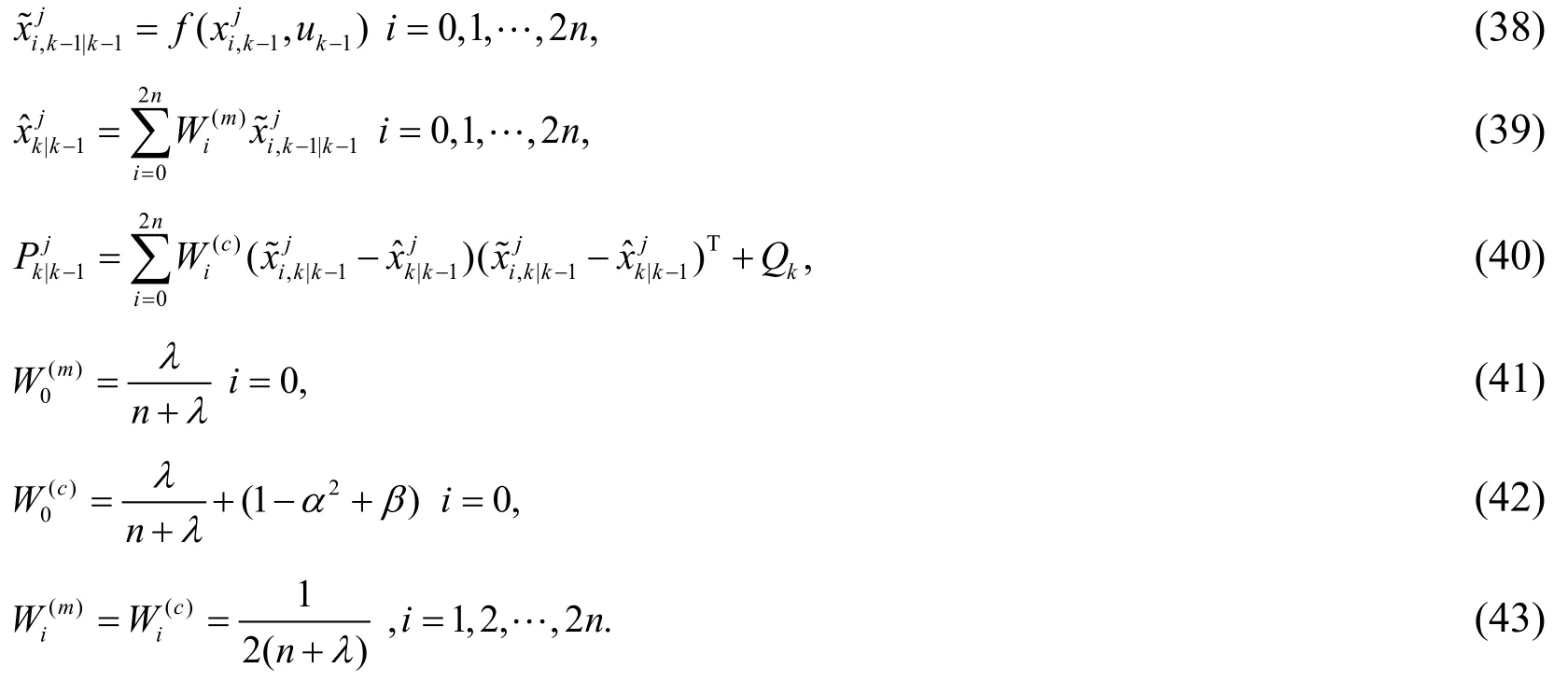
(c) Measure update

3) Model probability update

The model probability can be calculated by

4) Predicting combination

The combination result and its covariance at time k+1are

The final prediction ykIMMis probability-weighted sum of prediction from all models which are obtained in the data-driven model identification.

As it is shown in Fig. 1, the overall structure of the proposed predictor can be divided into three parts. Firstly, initial data set is used to train GP model and RELM model respectively. Secondly, the predicted values from initial GP model and RELM model are compared with predefined accuracy. If the accuracy meets the requirement, the predicted values can go into the IMM predictor directly. Otherwise, meaningful new data selected by data selection methods are introduced to update the GP model and RELM model recursively. Then new predicted values from updated models go into the IMM predictor.At the last part, the predicted values from different models are weighted according to the probability to obtain the final predicted values in IMM predictor.

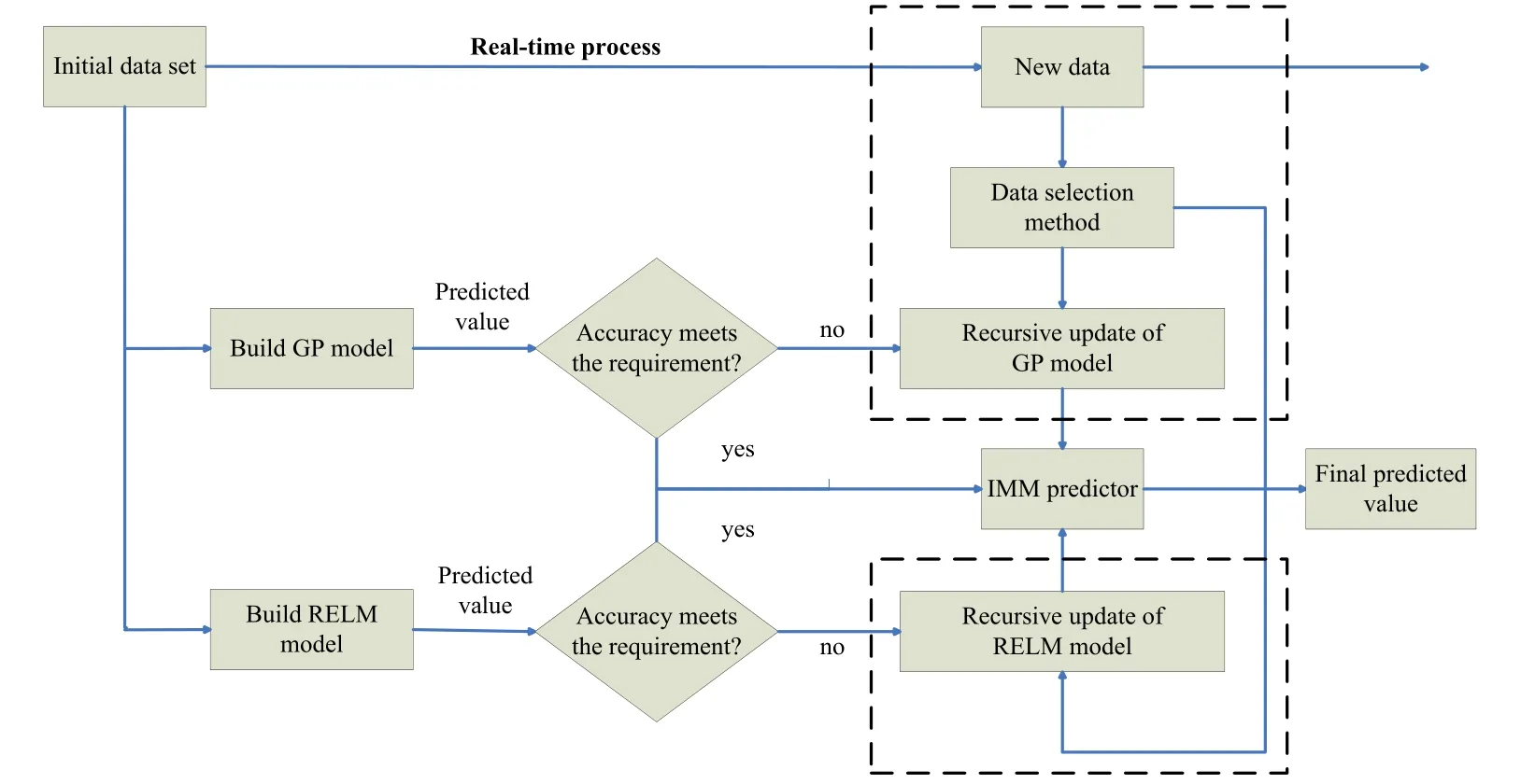
Figure 1: The overall structure of the proposed prediction method

5 Application to moisture content of ASP flooding

In this section, the characteristic of the proposed method and its application will be discussed. Firstly, the ASP flooding process is introduced. It is noted that we just list the one-dimensional model because three-dimensional model for ASP flooding that includes a series of divergence and cross terms, is too complex. The model for ASP flooding is

where a denotes the alkali,s denotes the surfactant,p denotes the polymer,Swis the water saturation,A is the core cross section area,fwis the moisture content,vwdenotes the seepage speed of water phase,Ca, Cs,Cpand Da, Ds,Dpdenote the concentration and diffusion coefficient of alkali, surfactant and polymer respectively.ρrdenotes the core density,Γa, Γs, Γpare the adsorbing capacity of core for different displacing agents,andRais the alkali consumption.

The aim is to build the relationship between moisture contentfwand injection concentration Ca, Cs,Cp. Obviously, it is a nonlinear dynamic system which is very difficult and time-consuming to solve the mechanism model for ASP flooding directly.So the data-driven identification model is built in this paper. The three-slug injection is adopted to calculate the moisture content in this case. The injection concentration is

where u=[ua, us, up]means the normalized injection concentration. In the identification model, the output is moisture content, represented asy, and the input vector is presented asx= [ y(k - 1),u(k)]. There are four injection wells with the same injection concentration,nine production wells, and the center of every four production wells is an injection well.The distribution of well position is shown in Fig. 2, where “S” means production well,“I” means injection well.

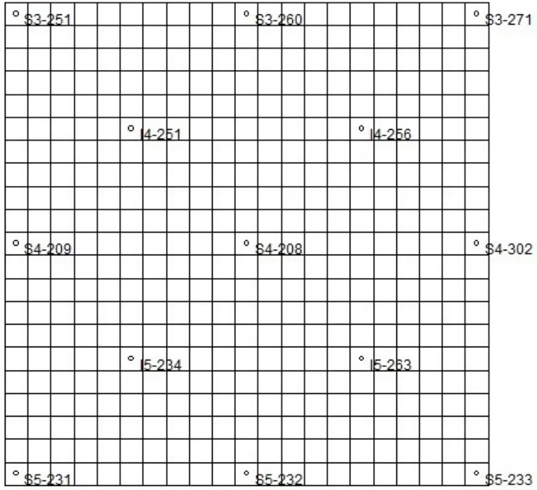
Figure 2: The distribution diagram of well positon

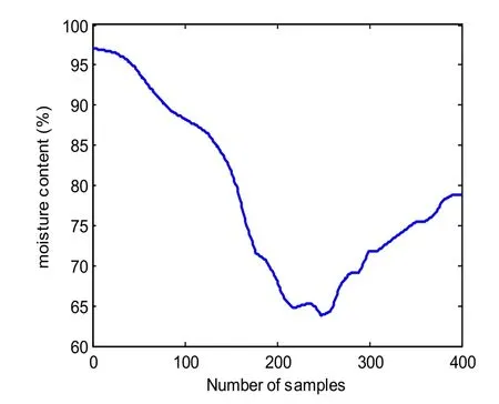
Figure 3: Moisture content data sets from production well S3-251

In this paper, the data from production well S3-251 is chose for model construction. In fact, data from other production wells can also be used for model construction. The moisture content can be calculated from reservoir simulation software CMG. About 1600 samples are obtained, one is retained every four samples, so 400 samples are left, where the first 200 is training data, the other 200 is testing data. Moreover, in order to model the real measure data more reasonable, the random white noise with appropriate size can be added to the final 400 samples. The final 400 samples are shown in Fig. 3 accompanied with corresponding injection concentration in Fig. 4.

The modeling performance is measured by the degree of agreement between the actual process and the model predicted output. In general, in order to show the efficiency of models, the comparison may be performed through visual inspection of the responses between the model and the process, then quantitatively evaluate the performance based on the values of selected performance indicators. The common performance indicators are root-mean-square error (RMSE) and relative root-mean-square error (RRMSE). If there areK elements, they are defined as

RMSE is a good measure of accuracy for a particular variable, but not between variables,because it is scale-dependent. RRMSE gives relative ratios without units, which are usually expressed as percentages. In addition, the absolute value of the relative error(ARE) is employed to evaluate the capability of model to track the trend of an evolving process.

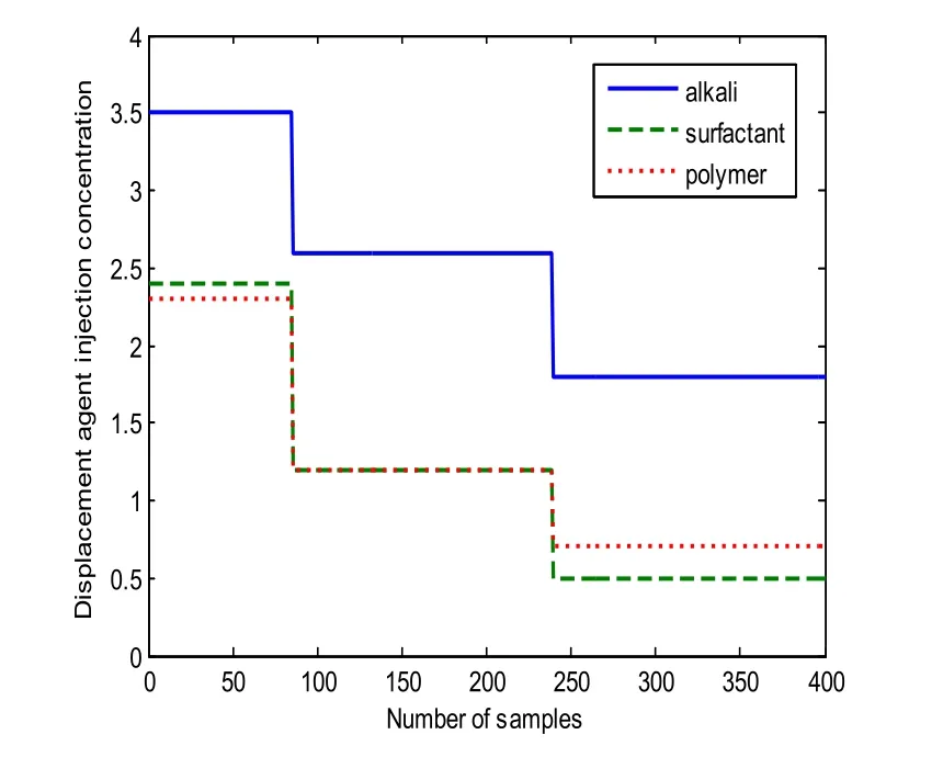
Figure 4: Displacement agent injection concentration for sample data

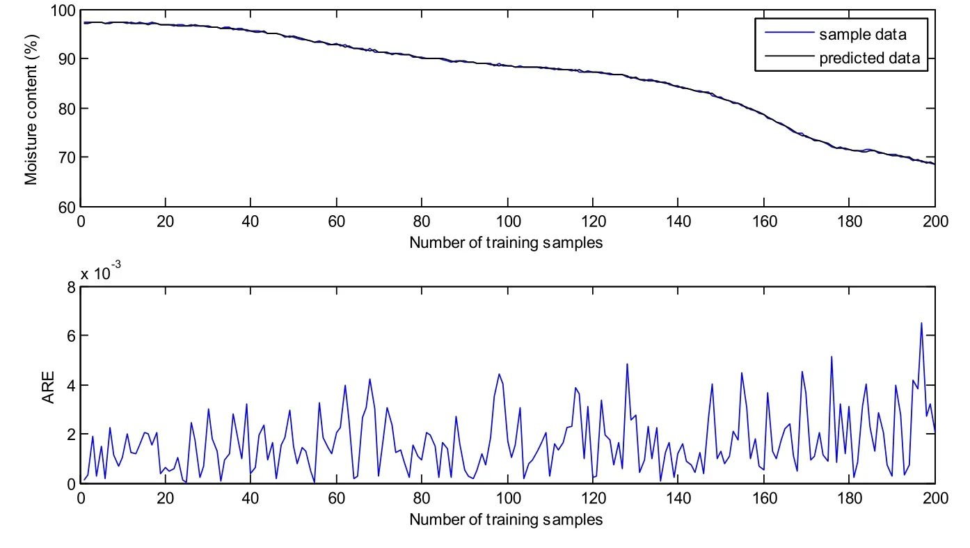
Figure 5: Predicted results of GP model on training samples

The first 200 samples are utilized to train the GP model. The training results are shown in Fig. 5. Most of the ARE are below 0.004, the RMSE and RRMSE are 0.1726 and 0.21%respectively. It is no doubt that the GP model matches the training samples very well. In order to verify the prediction performance, the obtained GP model is tested on the other 200 samples. Fig. 6 shows the predicted results of GP model on testing samples without update. It is clear that the predicted data curve gradually deviates from sample data curve at about the 40th testing sample. The predictive variance curve also appears a big rise at the same point, which means the prediction may be not accurate. In fact, it can be found from Fig. 4 that the control vector shows a sudden fall at about the 40th testing sample(the 240th sample). However, the training samples do not include the information of the sudden change of control vector. It can be seen that the changing operating conditions affect the prediction accuracy seriously. According to the proposed method, the predictive variance is above the variance limit, the corresponding data can be viewed as meaningful new data, which will be used to update GP model recursively. Fig. 7 demonstrates the predicted results after the first update with the addition of new data (the 240th sample). Compared with Fig. 6, the predictive variance becomes smaller, and the prediction performance improves a lot. If the predictive accuracy meets the accuracy requirements (predefined according to the practical situation), the update process will be terminated, otherwise other meaningful new data will be selected like the first one through the predictive variance until the accuracy requirements are met. Because the middle update processes are similar to the first one, so we do not enumerate here. The predicted results of GP on testing samples after the second update are demonstrated in Fig. 8. It is obvious that the predictive variances are all very small, denoting a high confidence level of the prediction. In addition, the RMSE and RRMSE of update process are listed in Tab. 1. It can be seen that the prediction performance has a big improvement after each update.

Table 1: RMSE and RRMSE of GP model for prediction

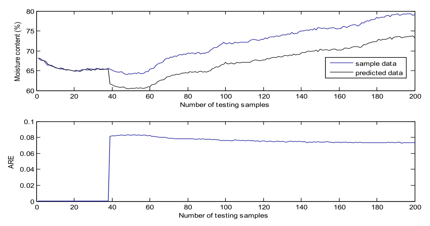
Figure 6: Predicted results of GP model on testing samples without update

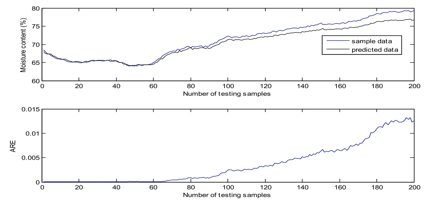
Figure 7: Predicted results of GP model on testing samples after the first update

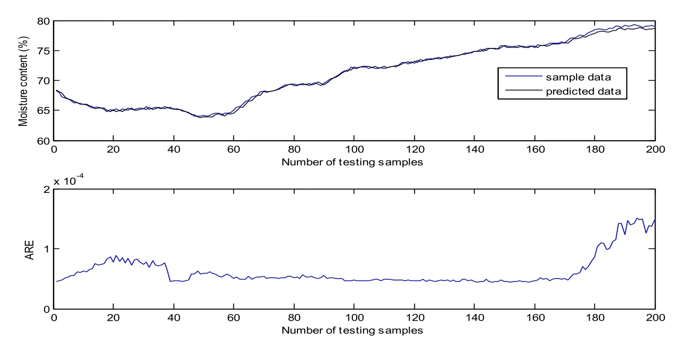
Figure 8: Predicted results of GP model on testing samples after the second update

The training results of RELM model is shown in Fig. 9. The model also shows a good match with the training samples. The RMSE and RRMSE are 0.2137 and 0.25%respectively. As shown in Fig. 10, a sudden change also occurs at about the 40th testing sample because of the same reason mentioned above. The difference is that predictive errors (ARE) become the measure of data selection. The predicted results of the first update and the second update are presented in Fig. 11 and 12, the other middle update processes are also omitted. The RMSE and RRMSE are summarized in Tab. 2. A similar conclusion can be drawn that the update improves the predictive accuracy greatly.

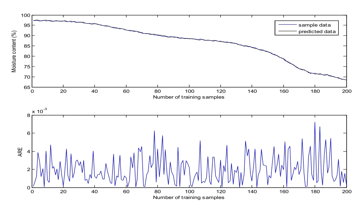
Figure 9: Predicted results of RELM model on training samples

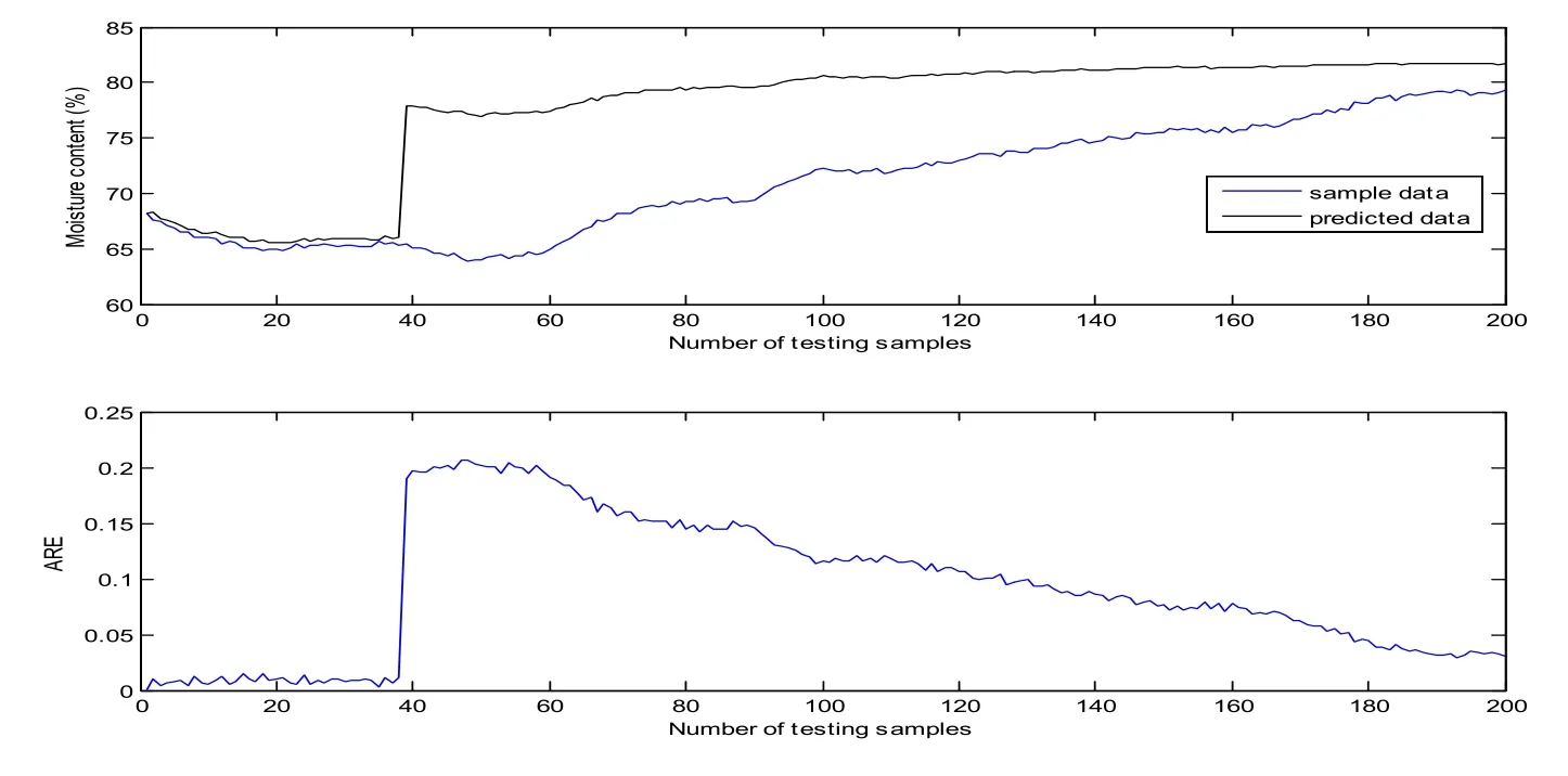
Figure 10: Predicted results of RELM model on testing samples without update

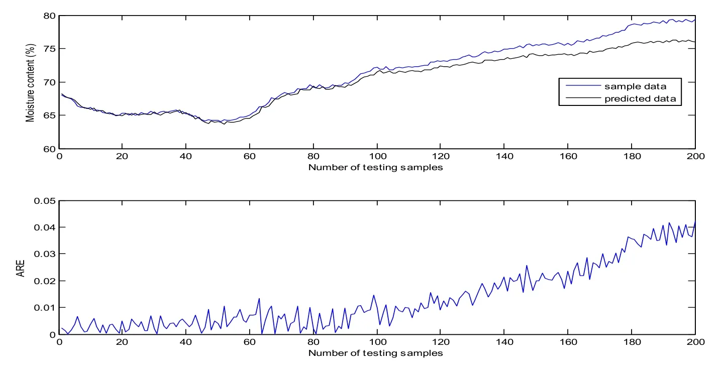
Figure 11: Predicted results of RELM model on testing results after the first update

When the final GP and RELM models are determined, they can be regarded as components of IMM predictor for a hybrid prediction. Fig. 13 illustrates the predicted moisture content curves of different models. And the corresponding RMSE and RRMSE are shown in Tab. 3. It demonstrates that IMM hybrid prediction shows better prediction performance on accuracy and robustness. In fact, adding meaningful new samples can reduce the impact from sudden changes of operating conditions, but it cannot break the limits from the model itself. Comparing with single-model prediction, hybrid prediction can combine the characteristics of different models and avoid the error accumulation resulting from single-model prediction.

Table 2: RMSE and RRMSE of RELM model for prediction

Table 3: RMSE and RRMSE of different models for prediction

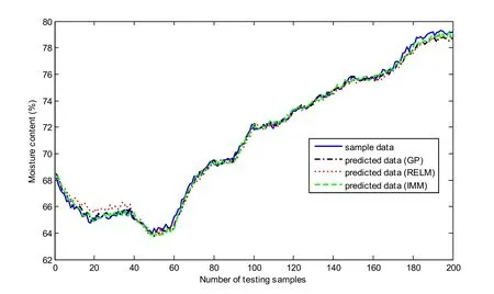
Figure 13: Predicted results of different models on testing samples

6 Conclusion

An interacting multiple-model prediction method is proposed and applied to moisture content of ASP flooding in this paper. Firstly, GP model and RELM model are used to model the process respectively on the basis of their own characteristics. The training results demonstrate that both models match the samples very well. However, the predictive accuracy may become bad when the operating conditions change. Thus,meaningful new sample data are incorporated into the models by recursive update. The testing results show the effectiveness of update strategies. Then, IMM algorithm is utilized for the hybrid prediction using the two models as components. The predicted results illustrate the hybrid prediction outperforms each single prediction on accuracy and robustness. The moisture content is a very important parameter in the process of oil development. It is no doubt that the proposed method can be viewed as an effective tool for moisture content prediction.

Acknowledgement: Authors would like to thank the associate editor and the anonymous referees for their valuable comments and suggestions. This work is supported by National Natural Science Foundation under Grant No. 60974039, National Natural Science Foundation under Grant No. 61573378, Natural Science Foundation of Shandong province under Grant No. ZR2011FM002, the Fundamental Research Funds for the Central Universities under Grant No. 15CX06064A.

Conflict of interest: The authors declare that there is no conflict of interest regarding the publication of this paper.

Ažman, K.; Kocijan, J. (2007): Application of gaussian processes for black-box modelling of Biosystems. ISA transactions, vol. 46, no. 4, pp. 443-457.

Chan, L. L. T.; Liu, Y.; Chen, J. (2013): Nonlinear system identification with selective recursive gaussian process models. Industrial & Engineering Chemistry Research, vol.52, no. 51, pp. 18276-18286.

Csató, L.; Opper, M. (2002): Sparse on-line gaussian processes. Neural computation,vol. 14, no. 3, pp. 641-668.

Deisenroth, M. P.; Rasmussen, C. E.; Peters, J. (2009): Gaussian process dynamic programming. Neurocomputing, vol. 72, no. 7, pp. 1508-1524.

Deng, W.; Zheng, Q.; Chen, L. (2009): Regularized extreme learning machine. 2009 IEEE Symposium on Computational Intelligence and Data Mining, pp. 389-395.

di Sciascio, F.; Amicarelli, A. N. (2008): Biomass estimation in batch biotechnological processes by bayesian Gaussian process regression. Computers & Chemical Engineering,vol. 32, no. 12, pp. 3264-3273.

Golub, G. H.; Van Loan, C. F. (2012): Matrix computations, vol. 3, JHU Press.

Gregorčič, G.; Lightbody, G. (2008): Nonlinear system identification: From multiple-model networks to Gaussian processes. Engineering Applications of Artificial Intelligence, vol. 21,pp. 7, pp. 1035-1055.

Gregorčič, G.; Lightbody, G. (2009): Gaussian process approach for modelling of nonlinear systems. Engineering Applications of Artificial Intelligence, vol. 22, no. 4, pp.522-533.

Huang, G. B.; Zhu, Q. Y.; Siew, C. K. (2006): Extreme learning machine: theory and applications. Neurocomputing, vol. 70, no. 1, pp. 489-501.

Hong, P. T.; Tran, V. T.; Yang, B. S. (2010): A hybrid of nonlinear autoregressive model with exogenous input and autoregressive moving average model for long-term machine state forecasting. Expert Systems with Applications, vol. 37, no. 4, pp. 3310-3317.

Keerthi, S.; Chu, W. (2005): A matching pursuit approach to sparse gaussian process regression. Advances in neural information processing systems, pp. 643-650.

Kocijan, J.; Likar, B. (2008): Gas-liquid separator modelling and simulation with gaussian-process models. Simulation Modelling Practice and Theory, vol. 16, no. 8, pp.910-922.

Li, D.; Xie, Q.; Jin, Q. (2015): Quasi-linear extreme learning machine model based nonlinear system identification. Proceedings of ELM-2014, Springer, vol. 1, pp. 121-130.

Li, X. L.; Jia, C.; Liu, D. X.; Ding, D. W. (2014): Adaptive control of nonlinear discrete-time systems by using os-elm neural networks. Abstract and Applied Analysis,pp. 1-11.

Ni, W.; Tan, S. K.; Ng, W. J.; Brown, S. D. (2012): Moving-window gpr for nonlinear dynamic system modeling with dual updating and dual preprocessing. Industrial &Engineering Chemistry Research, vol. 51, no. 18, pp. 6416-6428.

O’Hagan, A.; Kingman, J. (1978): Curve fitting and optimal design for prediction.Journal of the Royal Statistical Society: Series B (Methodological), pp. 1-42.

Qi, C.; Li, H. X. (2008): A karhunen-Loève decomposition-based wiener modeling approach for nonlinear distributed parameter processes. Industrial & Engineering Chemistry Research,vol. 47, no. 12, pp. 4184-4192.

Qi, C.; Li, H. X. (2009): A time/space separation-based hammerstein modeling approach for nonlinear distributed parameter processes. Computers & Chemical Engineering, vol.33, no. 7, pp. 1247-1260.

Rasmussen, C. E. (1996): Evaluation of Gaussian processes and other methods for nonlinear regression (Ph.D. thesis). Citeseer.

Rasmussen, C. E.; Nickisch, H. (2010): Gaussian Processes for Machine Learning(GPML) Toolbox. Journal of Machine Learning Research, vol. 11, no. 6, pp. 3011-3015.

Seeger, M.; Williams, C.; Lawrence, N. (2003): Fast forward selection to speed up sparse gaussian process regression. Artificial Intelligence and Statistics.

Shao, Z.; Er, M. J. (2016): An online sequential learning algorithm for regularized extreme learning machine. Neurocomputing, vol. 173, pp. 778-788.

Shutang, G.; Qiang, G. (2010): Recent progress and evaluation of asp flooding for eor in daqing oil field. SPE EOR Conference at Oil & Gas West Asia, Society of Petroleum Engineers.

Tang, Y.; Li, Z.; Guan, X. (2014): Identification of nonlinear system using extreme learning machine based hammerstein model. Communications in Nonlinear Science and Numerical Simulation, vol. 19, no. 9, pp. 3171-3183.

Toh, K. A. (2008): Deterministic neural classification. Neural computation, vol. 20, no. 6,pp. 1565-1595.

Wang, M.; Qi, C.; Yan, H.; Shi, H. (2016): Hybrid neural network predictor for distributed parameter system based on nonlinear dimension reduction. Neurocomputing,vol. 171, pp. 1591-1597.

Wang, M.; Yan, X.; Shi, H. (2013): Spatiotemporal prediction for nonlinear parabolic distributed parameter system using an artificial neural network trained by group search optimization. Neurocomputing, vol. 113, pp. 234-240.

Wang, Y.; Wang, J.; Wei, X. (2015): A hybrid wind speed forecasting model based on phase space reconstruction theory and markov model: A case study of wind farms in northwest china. Energy, vol. 91, pp. 556-572.

Yan, W.; Shao, H.; Wang, X. (2004): Soft sensing modeling based on support vector machine and Bayesian model selection. Computers & Chemical Engineering, vol. 28, no.8, pp. 1489-1498.

Zerpa, L. E.; Queipo, N. V.; Pintos, S.; Salager, J. L. (2005): An optimization methodology of alkaline-surfactant-polymer flooding processes using field scale numerical simulation and multiple surrogates. Journal of Petroleum Science and Engineering, vol. 47,no. 3, pp. 197-208.

Zhang, Y. (2011): Hourly traffic forecasts using interacting multiple model (imm)predictor. IEEE Signal Processing Letters, vol. 18, no. 10, pp. 607-610.