Study on segmented distribution for reliability evaluation

Li Huaiyuan,Zuo Hongfu,Su Yan,Xu Juan,Yin Yiing

aSchool of Software Engineering,Jinling Institute of Technology,Nanjing 211169,China

bCollege of Civil Aviation,Nanjing University of Aeronautics and Astronautics,Nanjing 211106,China

Study on segmented distribution for reliability evaluation

Li Huaiyuana,b,Zuo Hongfub,*,Su Yanb,Xu Juanb,Yin Yibingb

aSchool of Software Engineering,Jinling Institute of Technology,Nanjing 211169,China

bCollege of Civil Aviation,Nanjing University of Aeronautics and Astronautics,Nanjing 211106,China

Bayesian estimates;Gibbs sampling method;Maximum likelihood estimation;Proximity sensors in leadingedge flap in aircraft;Reliability;Segmented distribution;Weibull distribution

In practice,the failure rate of most equipment exhibits different tendencies at different stages and even its failure rate curve behaves a multimodal trace during its life cycle.As a result,traditionally evaluating the reliability of equipment with a single model may lead to severer errors.However,if lifetime is divided into several different intervals according to the characteristics of its failure rate,piecewise fitting can more accurately approximate the failure rate of equipment.Therefore,in this paper,failure rate is regarded as a piecewise function,and two kinds of segmented distribution are put forward to evaluate reliability.In order to estimate parameters in the segmented reliability function,Bayesian estimation and maximum likelihood estimation(MLE)of the segmented distribution are discussed in this paper.Since traditional information criterion is not suitable for the segmented distribution,an improved information criterion is proposed to test and evaluate the segmented reliability model in this paper.After a great deal of testing and verification,the segmented reliability model and its estimation methods presented in this paper are proven more efficient and accurate than the traditional non-segmented single model,especially when the change of the failure rate is time-phased or multimodal.The significant performance of the segmented reliability model in evaluating reliability of proximity sensors of leading-edge flap in civil aircraft indicates that the segmented distribution and its estimation method in this paper could be useful and accurate.

1.Introduction

As one of the essential devices affecting aircraft safety,the proximity sensors in leading-edge flap is an important part of aircraft operating system.However,proximity sensors in leading-edge flap are also one of the devices with higher failure rate in aircraft.1In order to ensure aircraft safety and reduce its maintenance costs,it’s necessary to accurately evaluate the reliability of proximity sensors in leading-edge flap.2However,like most other equipment,the failure rate of the proximity sensors in leading-edge flap is complicated,exhibiting different changes in different operation phases.3In order to accurately evaluate the reliability of devices such as proximity sensors in leading-edge flap,whose failure rate is multimodal or multi-stage,only segmented distribution is applicable and inevitable.4In this paper,two segmented reliability models are proposed:(1)failure rate is a piecewise linear function about lifetime,namely,segmented linear failure rate mode and(2)failure rate in any stage is of the same formula as the failure rate function of Weibull distribution,called segmented Weibull distribution.

Currently,the application of segmented distribution to reliability evaluation is mainly classified into three categories:describing the degradation process of devices;creating reliability model;and testing and detecting change-points.5(1)Now,how to fit the equipment degradation process by segmented distribution is discussed in a lot of literature.For example,Bae et al.6proposed a hierarchical Bayesian change-point regression model to fit two-phase degradation patterns and derived the failure-time distribution of a unit randomly selected from its population.Kvam7introduced a log-linear model with random coefficients and a change-point to describe the nonlinear degradation path.(2)Since the failure rates of many products may perform different trends at different stages,an application of segmented distribution to evaluating product reliability has been widely concerned.Li et al.8estimated the change-point for a piecewise hazard regression model in the presence of right censoring and long-term survivors.In a study by He et al.9,a sequential testing approach to detect multiple change-points in the hazard function by likelihood ratio statistics and resampling was proposed,which was applicable to both right-censored and interval-censored data.Uhm et al.10studied a weighted least squares estimator for Aalen’s additive risk model with right-censored survival data which may allow for very flexible handling of covariates.(3)In addition,another important application of segmented distribution is to test whether there are change-points in product failure rate or reliability.For a segmented regression system with an unknown change-point over two domains of a predictor,a new empirical likelihood ratio statistic was proposed to test the null hypothesis of no change by Liu and Qian11.Goodman et al.12expanded the set of alternatives to allow for multiple change-points,and proposed a model selection algorithm using sequential testing for the piecewise constant hazard model.Suresh13derived a test statistic and its asymptotic distribution,and compared the power of the test with other existing tests such as likelihood ratio,Weibull,and log Gamma tests.Nosek and Szkutnik14discussed a regression model with a possiblestructuralchangeand a smallnumberof measurements.

Recently,segmented distribution and its estimation method have caught more attentions.To minimize the expected sum of manufacturing cost,bum-in cost,and warranty cost of failed items found during their warranty period,a cost model was formulated to find the optimal bum-in time based on Weibull hyperexponential distribution by Chou and Tang15.Considering different prior densities for parameters and censored survival data,Achcar and Loibel16discussed Bayesian analysis on segmented constant hazard function models and put forward their inference methods by Metropolis algorithms.Weibull-exponential distribution,a common segmented distribution,was discussed and its accurate calculation formula by Bayes estimation was proposed by Boukai17.Patra and Dey18proposed a general class of change-point hazard models for survival data,which included and extended many different types of segmented distribution.

However,the existent segmented distribution is generally considered as a two-segment distribution,or their failure rate is supposed as a constant in recent literature6–18.Compared with many other current segmented distributions,the contributions of this paper are as follows.(1)In this paper,not only two kinds of universaln-segment distribution have been discussed,but also two general methods to estimate parameters in the segmented distributions,namely Bayesian estimation and maximum likelihood estimation(MLE),are given.(2)An information criterion adequate for then-segment distribution is proposed.It can not only test whether a change-point exists or not,but also measure the appropriateness and correctness of the segmented reliability model.(3)A new bathtub curve model is put forward to verify the effects of the segmented distributions.

2.Segmented distribution

In fact,the failure rate of equipment not only is changeable but also often manifests different trends at different phases.Reliability-centered maintenance(RCM)recommended six failure models as shown in Fig.1.19As Fig.1 shows,apart from failure models C and E,the failure rates of the other failure models show different patterns at different phases,and change-points obviously exist in failure rate curves.Therefore,if one and same distribution is utilized to evaluate a failure whose failure rate is characterized by multiple change-points and multi-peak,evaluation may be rather difficult and inaccurate.20

Due to unevenness and inconsistency of failure rate,it is not appropriate to describe the change of reliability by one and same analytical function in the entire lifetime cycle.However,if we divide lifetime into some time intervals according to failure rate trend,the failure rate in every different interval can be described by a different function.Just as piecewise interpolation with a simple function can improve approximation precision,we can more accurately approximate the true change of failure rate.For example,as for failure model A,i.e.,bathtub curve,if three different failure rate functions are in correspondence to each phase,then the change of failure rate in the entire lifetime cycle of equipment can be accurately fitted by segmented distribution.

Supposingthatlifetimeisdividedintonintervalsandthefailureratefunctioninthei-thinterval[τi，τi+1)isexpressedbyhi(t),thenthesegmentedfailureratefunctionh(t)canbeexpressedby Eq.(1)below,wherehi(t)＞ 0,t∈ [τi，τi+1)is requisite.

Furthermore,fi(t)andRi(t)can piecewise compose the segmented probability density functionf(t)and the reliability functionR(t)in the entire lifetime cycle,shown as Eqs.(6)and(7),respectively.

2.1.Segmented linear failure rate model

2.1.1.n-segment linear failure rate model

As calculation of piecewise linear interpolation is easy and can meet most engineering requirements,we divide lifetime intonintervals and set the failure rate functionhi(t)in thei-th interval[τi，τi+1)as Eq.(8),where μi≤ τiis required.Usually,μi=0 or μi= τi.According to Eqs.(2)and(3),we getJiandKi(t),shown as Eqs.(9)and(10),respectively.

Furthermore,according to Eqs.(6)–(10),we can obtain the probability density functionfi(t)and the reliability functionRi(t)in thei-th interval,respectively,shown as Eqs.(11)and(12).

If βi＞ 0,then the failure rate in thei-th interval will linearly increase;if βi=0,the failure rate in thei-th interval will be constantly kept as αi;if βi＜ 0,then the failure rate in thei-th interval will linearly decrease.Ift∈ [tn，∞),then βn＞ 0 is required in order to ensurehn(t)＞ 0，t∈ [tn，∞).However,ifh(t)is defined in finite support on some special occasions,βn≤ 0 may be acceptable.

2.1.2.Linear failure rate model

Particularly,if lifetime isn’t segmented,namely,nonsegmented,then the failure rate will linearly change in the entire lifetime cycle.h(t),f(t)andR(t)of the linear failure rate mode are expressed as Eqs.(13)–(15),respectively.

Fig.2 shows some typical function curves of this distribution,from which we can see that μ1and τ1can adjust the curve shape and its starting point.Specially,when β1=0 and μ1= τ1, the distribution will become an exponential distribution.

2.1.3.Two-segment linear failure rate model

In general,n=2 orn=3,namely two-or three-segment distribution can meet most of reliability evaluation.For twosegment distribution,h(t)andR(t)will be Eqs.(16)and(17),respectively.Supposing that μ1= τ1=0, μ2= τ2=1.5,some curves of the two-segment linear failure rate model are shown in Fig.3.From Fig.3,it can be seen that the segmented distribution may degenerate into a non-segmented mode when the failure rate changes consistently and continuously in the entire lifetime cycle.When the failure rate changes in an obviously phased manner,this segmented distribution can also precisely reflect the different changes of the failure rate in its every interval.

2.1.4.Three-segment linear failure rate model

Whenn=3,h(t)andR(t)of the three-segment linear failure rate model are respectively shown as Eqs.(18)and(19).When μ1= τ1=0,μ2= τ2and μ3= τ3=2.5,some function curves of the three-segment linear failure rate model are shown in Fig.4.From Fig.4,it’s clear that the adaptability of segmented distribution is extensive,as it can express both the case where the failure rate changes sharply and the case where the failure rate has no obvious change when αi≈ αi+1，βi≈ βi+1.From Figs.3 and 4,it’s apparent thatf(t)seems more fluctuating when the trend of the failure rate is obviously in a staged or piecewise manner.

2.2.Segmented Weibull distribution

Although then-segment linear failure rate functionh(t)can express the change of failure rate in a staged manner,it can only express a linear relation.Meanwhile,linear fitting is not precise enough and its adaptability is not good enough.Never-theless,by adjusting shape parameters,Weibull distribution can not only express a distribution with an increasing failure rate,but also model a distribution whose failure rate is decreasing.21,22Therefore,the failure rate in each interval is fitted by Weibull failure rate functions with different parameters,and better precision and adaptability can be achieved.23,24

2.2.1.n-segment Weibull distribution

Let the failure rate functionhi(t)in thei-th interval[τi，τi+1)be Eq.(20).From Eqs.(2)and(3),we obtainJiandKi(t),respectively shown as Eqs.(21)and(22).

Here μi≤ τi，αi＞ 0，βi＞ 0. Furthermore, according to Eqs.(6),(7)and(20)–(22),the probability density functionfi(t)and the reliability functionRi(t)in thei-th interval are respectively obtained as Eqs.(23)and(24).

If βi＞ 1,thenhi(t)increases in the interval[τi，τi+1);if βi=2,thenhi(t)becomes a linearly increasing function;if βi=1,thenhi(t)is fixed at αiin the interval[τi，τi+1);if βi＜ 1,thenhi(t)decreases in the interval[τi，τi+1).In this way,the segmented Weibulldistribution can flexibly approximate the changefulfailure rate.If lifetime is non-segmented,it will become a classical Weibull distribution.Usually,the segment numbern≤3 can satisfy the requirement of reliability evaluation in most cases.

2.2.2.Two-segment Weibull distribution

In particular,if lifetime is divided into two intervals,according to Eqs.(23)and(24),h(t)，f(t)andR(t)of the two-segment Weibull distribution are respectively shown as Eqs.(25)–(27).Let μ1= τ1=0,some curves of the two-segment Weibull distribution are drawn in Fig.5.

2.2.3.Three-segment Weibull distribution

Similarly,whenn=3,thenh(t)andR(t)of the three-segment Weibull distribution can be respectively written as Eqs.(28)and(29).When μ1= τ1=0,some three-segment curves of the Weibull distribution are shown in Fig.6.

From Figs.5 and 6,the segmented Weibull distribution can precisely approximate the sharp fluctuation of failure rate.As for multimodal distribution or varying failure rate,such as bathtub curve,the segmented Weibull distribution is very appropriate.

However,if the parameters in the segmented distribution are not appropriate,f(t)of the segmented distribution att=τimay incur a discontinuity point.For example,when μi= τi,h(t)andf(t)of the segmented Weibull distribution att=τiare discontinued,but this discontinuity may not affect the measurement of reliability,becauseR(t)is continuous.As a whole,the segmented distribution in this paper can be fit to all kinds of failure mode recommended by RCM.

3.Estimation of segmented distribution

If the sample setS= ｛t1，t2，...，tk，...，tm｝ of segmented distribution is known,in order to estimate parameters in segmented distribution,we should,first of all,estimate change-points τ1，τ2，...，τnand location parameters μ1，μ2，...，μn.25Usually,let μi=0(i=1，2，...，n)or μi= τi(i=1，2，...，n).Of course,there are many other more accurate methods to estimate μiand τi.In this paper,Bayesian estimation and MLE are utilized to preliminarily estimateparametersin segmented distribution.26

3.1.Bayesian regression estimation of segmented distribution

Usually,a piecewise-linear regression model is defined as Eq.(30).Namely,the response of any inputxj∈ [τi，τi+1)contains two terms:the linear functionai+bixjand the stochastic disturbance εithat obeys normal distributionN(0，σ2i).The aim of piecewise-linear regression is to infer parametersaiandbiunder the circumstance thatminput samplesxjand their correspondingly output samplesyjare known.Denoted by a=(ai)n×1,b=(bi)n×1, σ2=(σ2i)n×1, τ=(τi)n×1,X=(xi)m×1,Y=(yi)m×1,under the condition that parameters a，b，σ2and τ are given,then the maximum likelihood function ofnsegment distribution is written as Eq.(31).In addition,the residual sum of squaresQin Eq.(32)can re flect precision of fitting.

3.1.1.Prior distribution of Bayesian regression

Usually,properly determining prior distribution is a key of Bayesian estimation.Althoughai,bi,σ2i,τiin most Bayesian estimation are supposed to be independent27,28,in fact,there are close relations amongai,bi,σ2i,τi.

Proof.From Eq.(30),ifxj1∈ [τi，τi+1)，xj2∈ [τi，τi+1),then their stochastic disturbances εj1and εj2will also obey normal distributionN(0，σ2i),namely,

Thus,we get

Furthermore,if any two samples are combined,then summation of all combinations will also obey normal distribution,i.e.,

After deduction and simpli fication,it’s concluded thatbiobeys normal distribution when σ2i，τ are given,namely,

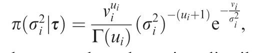
Theorem 3.Assuming thatπ(τi)is the prior distribution ofτi;the distribution ofσ2

i|τis denoted asπ(σ2i|τ)under the conditionthatτis given;and parameters ai,bi,σ2i,τiin the ith segment are independent from parameters aj,bj,σ2j,τjin the jth segment,then the prior distribution of the piecewise-linear regression model inEq.(30)can be written as

Proof.From the topic supposes,as the parameters in different segments are independent of each other,we get

From Theorems 1 and 2,the prior distribution of the model in Eq.(30)is obtained as Eq.(33).Unlike other linear regression models,the above prior distribution in Theorem 3 can express relations among parametersai，bi，σ2i，τi.□

Usually,inverse Gamma distribution IG(ui，vi)or uniform distributionU(ui，vi)or non-information distribution can be taken as a prior distribution of σ2i|τ.If samplesxjandyjhave been correctly divided,namely τ is known,the following Algorithm 1 can estimate hyper-parametersuiandviof thei-th segment.

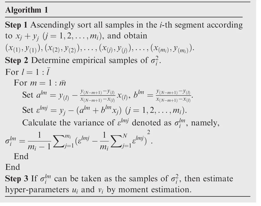
Algorithm 1 Step 1 Ascendingly sort all samples in the i-th segment according to xj+yj(j=1，2，...，mi),and obtain(x(1)，y(1))，(x(2)，y(2))，...，(x(j)，y(j))，...，(x(mi)，y(mi)).Step 2 Determine empirical samples of σ2 i.For l=1:¯l For m=1:¯m Set alm=y(l)-x(N-m+1)-x(l)x(l),blm=y(N-m+1)-y(l)y(N-m+1)-y(l)x(N-m+1)-x(l).Set εlmj=yj-(alm+blmxj)(j=1，2，...，mi).Calculate the variance of εlmjdenoted as σlmi,namely,2 σlmi=11 mi-1∑mi j=1(εlmj-mi∑N j=1εlmj).End End Step 3 If σlmican be taken as the samples of σ2i,then estimate hyper-parameters uiand viby moment estimation.

The prior distribution of change-points τi,denoted as π(τi),is often considered as a discrete distribution de fined in samplesxi(i=1，2，...，m).16The greater the first-and second-order differences of(xj，yj)are,the higher the probability that change-points occur atxjwill be,and thus it should be atxjthat samples are divided.In this paper,the flow of determination of π(τi)is shown as the following Algorithm 2.

3.1.2.Bayesian piecewise-linear regression estimation

Algorithm 2 Step 1 Ascendingly sort all samples(xj，yj)according to xj(j=1，2，...，m)and get(x(1)，y(1))，(x(2)，y(2))，...，(x(j)，y(j))，...，(x(m)，y(m)).Step 2 Set∂′j=y(j+1)-y(j-1)x(j+1)-x(j-1)(j=2，3，...，m-1),∂′1=0,∂′m =0,and then normalize∂′j,namely set p′j=∑m i=1|∂′|∂ ′j|i|.Step 3 Set∂′′j=j+1-∂′j-1 x(j+1)-x(j-1)∂′(j=2，3，...，m-1),∂′′1=0,∂′′m=0,and then normalize∂′′j,namely set p′′j=∑m i=1|∂′′i|.|∂′′j|Step 4 Calculate wj.When m is an even number,set wj=■■■ ■■4(j-1)m(m-2) j=1，2，...，m2 4(m-j)m(m-2)j=m ;when m is an odd m 2+2，...，m 2+1，m+1 2 number,set wj=■■■ ■■4(j-1)(m-1)2j=1，2，...，4(m-j)(m-1)2j=m+3 2 ，m+5 2 ，...，m.（■ ■）（ ）■ ■Step 5 Set lπi=max 1，(i-2),and get the prior distribution m n ,rπi=min m，im n π(τi=xj)=■■ ■∑rπii) j=lπi，lπi+1，...，rπi 0 Others wj(p′j+p′′j)i=lπiwi(p′i+p′′j=1，2，...，m;i=2，3，...，n.

In Algorithm 2,Step 4 ensures that the middle samples are more likely to be regarded as τi,which is inclined to make all segmentation as equalized as possible.In addition, π(τ1)and π(τn+1)are deemed as constants,for example,its distribution may be often written as the following formula.

Eq. (35) merely includes hyper-parametersui,vi(i=1，2，...，n);however,the posteriori distribution of parameters is difficult to be explicitly expressed.Therefore,it must be the Gibbs sampling method is utilized to find out its numerical solution.

Theorem 4.In the joint distribution in Eq.(35),if parameters al,b,σ2,τand samplesX，Yare given,then the full conditional distribution of parameters ai(i≠l)will obey normal distribution,namely,

Proof.ifal，b，σ2，τ，X，Y，l≠iin Eq.(35)are fixed,then we obtain

is obtained.Furthermore,we get

Obviously,it is a kernel of normal distribution.Thus we get

Theorem 5.In the joint distribution in Eq.(35),if parametersa,bl,σ2,τand samplesX,Yare given,then the full conditional distribution of parameters bi,i≠l will obey normal distribution,namely,

Proof.Supposing that X,Y,a,bl,σ2,τ,l≠iin Eq.(35)are constants,then we get

After derivation and simplification,we get

In addition,because it’s easy to know

is obtained.Obviously,it is also a kernel of normal distribution.Therefore,we get

Proof.Supposing that a,b,σ2l,τ,X,Y in Eq.(35)are constant,then we get

After further derivation and simplification,we get

Therefore,it’s tenable that

Theorem 7.In the joint distribution in Eq.(35),if parametersa,b,σ2,τland samplesX,Yare given,then the full conditional distribution ofτi|a，b，σ2，τl，X，Yabout parametersτi(i≠l)is same as the prior distributionπ(τi),namely,

Proof.Similarly,if parameters a,b,σ2,τl,X,Y in Eq.(35)are deemed as constants,then we obtain

Because π(τi)is a discrete distribution,we get

According to the above full conditional distribution,if the model in Eq.(30)is inferred by Bayesian estimation,then the Gibbs sampling method is shown as the following Algorithm 3.

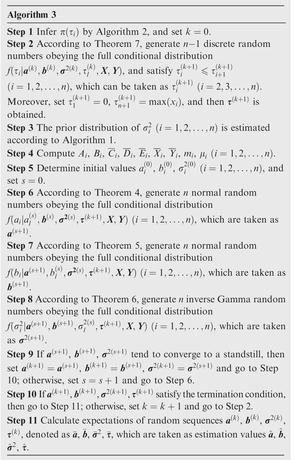
Algorithm 3 Step 1 Infer π(τi)by Algorithm 2,and set k=0.Step 2 According to Theorem 7,generate n-1 discrete random numbers obeying the full conditional distribution f(τi|a(k)，b(k)，σ2(k)，τ(k)l ，X，Y),and satisfy τ(k+1)i ≤ τ(k+1)i+1(i=1，2，...，n),which can be taken as τ(k+1)i (i=2，3，...，n).Moreover,set τ(k+1)1 =0,τ(k+1)n+1 =max(xi),and then τ(k+1)is obtained.Step 3 The prior distribution of σ2i(i=1，2，...，n)is estimated according to Algorithm 1.Step 4 Compute Ai,Bi,Ci,Di,Ei,Xi,Yi,mi,μi(i=1，2，...，n).Step 5 Determine initial values a(0)i,b(0)i,σ2(0)i (i=1，2，...，n),and set s=0.Step 6 According to Theorem 4,generate n normal random numbers obeying the full conditional distribution f(ai|a(s)l ，b(s)，σ2(s)，τ(k+1)，X，Y)(i=1，2，...，n),which are taken as a(s+1).Step 7 According to Theorem 5,generate n normal random numbers obeying the full conditional distribution f(bi|a(s+1)，b(s)l ，σ2(s)，τ(k+1)，X，Y)(i=1，2，...，n),which are taken as b(s+1).Step 8 According to Theorem 6,generate n inverse Gamma random numbers obeying the full conditional distribution f(σ2i|a(s+1)，b(s+1)，σ2(s)l ，τ(k+1)，X，Y)(i=1，2，...，n),which are taken as σ2(s+1).Step 9 If a(s+1),b(s+1),σ2(s+1)tend to converge to a standstill,then set a(k+1)=a(s+1),b(k+1)=b(s+1),σ2(k+1)= σ2(s+1)and go to Step 10;otherwise,set s=s+1 and go to Step 6.Step 10 Ifa(k+1),b(k+1),σ2(k+1),τ(k+1)satisfytheterminationcondition,then go to Step 11;otherwise,set k=k+1 and go to Step 2.Step 11 Calculate expectations of random sequences a(k),b(k),σ2(k),τ(k),denoted as¯a,¯b,¯σ2,¯τ,which are taken as estimation values^a,^b,^σ2,^τ.

Under the same parameters circumstance,compute 1024 groups of simulation sample set.The average results are compared with those of other methods so as to verify the effects of the algorithms in this paper.In simulation verification,setn=1,a=-2,b=2,σ2=0.1,τ=0,μ =0 in Eq.(30).Then setm=16,namely,every 16 pairs random number(xj，yj)compose one group sample set.Simulation results are listed in Table 1.The results of non-information and uniform prior distributions are also tabulated in Table 1.

Fig.7 is a scatter diagram illustrating all sampling samples in a certain simulating calculation,which shows that the sampling samples are concentratedly distributed in the neighborhood of the true values of parameters.

Fig.8 illustrates sampling samples in course of iteration,which implies the algorithm begins to converge only at a cost of small quantity of iteration.

Assuming that parameters and their estimated values are respectively denoted as θ=(a，b，σ2)and^θ=(^a，^b，^σ2),then υ= ‖^θ - θ‖/‖θ‖ can reflect estimation accuracy.Qin Eq.(32)can measure fitting precision.In addition,iterationskcan imply algorithm efficiency.Therefore,the averages ofk,υ,Qfrom all simulating calculations,denoted asE(k),E(υ),E(Q),can indicate the effectiveness and efficiency of Algorithm 3.From Table 1,the effectiveness and efficiency of the algorithm in this paper are satisfying,because the relations among parameters are fully considered.

3.1.3.Bayesian regression estimation of segmented distributionIn thispaper,estimation ofsegmented distribution by Bayesian regression is based on the following hypotheses:(1)μiare given or known and(2)parametersai,bi,σ2i,τiin thei-th segment are independent of parametersaj,bj, σ2j, τjin thej-th segment.Usually,these hypotheses can be met in most practical cases.

Assuming that failure rate is linear,shown as Eq.(8),according to Eq.(36),Eq.(8)can be transformed into a linear relationshipy=ai+bix,which can meet the requirements of regression.If the estimation values ofai,biwith the Bayesian regression model are denoted as^ai,^bi,then^αi=^ai,^βi=^biare achieved.

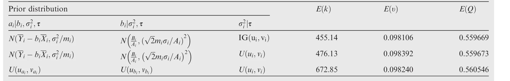
Table 1 Results of Bayesian estimation in simulation.

Thus,the failure rateh(tj)of sampletjis inferred firstly,and then(tj，h(tj))is transformed into sample(xj，yj)according to Eqs.(36)and(37).Next,regression coefficients can be estimated by Algorithm 3.In the end,the regression coefficients are transformed into parameters of segmented distribution.

3.2.MLE of segmented distribution

The unknown parameters in thei-th interval are written as θi=[αiβiμi]T.Supposing thatn,τi(i=1，2，...，n)are known,then the likelihood functionL(θ)ofn-segment distribution is written as Eq.(38)according to Eq.(6).Taking the logarithm ofEq.(38),wegetitslogarithmiclikelihoodfunctionlnLshown as Eq.(39).We take the partial derivative of Eq.(39)with respect to θi,which is the parameter in thei-th interval,and get Eq.(40).

3.2.1.Test change-points by improved information criterionUsually,only when the sample number of each interval is approximately equal or the difference among the lengths of different intervals is slight,partitioning is most reasonable.29,30In addition,the lower the number of interval is,the more concise the model will be.31In order to measure the appropriateness of segmented distribution,learning from the idea that the information criterion SIC penalizes the complexity of a model,the information criterion SIC is improved.Thus a novel information criterion ICSD appropriated for segmented distribution is proposed in this paper,which is shown as Eq.(43).32,33In Eq.(43),lnL(θ)means the logarithm likelihood function shown as Eq.(39);θ are the unknown parameters to be estimated;anddθis the dimensions of unknown parameters θ;mis the total number of samples;nis the number of intervals,i.e.,the segmentation number;cpenaltyis the penalty item expressed by the standard deviation,which is calculated by Eq.(41)or(42).In Eq.(41),miindicates the sample number of thei-th interval;τn+1in Eq.(42)is usually supposed as the maximum sample,and of course,there are other methods to estimate τn+1.In the special case ofn=1,Eq.(43)is exactly the same as SIC information criterion.34Therefore,whennand τiare given,the MLE of then-segment distribution can be taken as an optimization problem,which is shown as Eq.(44).

Eq.(44)can also be utilized to test whether change-points exist or not.Namely,min ICSDτi，n(θ) ＜ SIC indicates that there obviously exist some change-points and estimating by the segmented distribution is appropriate.Let Eq.(40)be 0,we can get likelihood equations.Although the solution of likelihood equations can be regarded as an estimation of unknown parameters,usually we may get no solution at all or multiple solutions due to the too high complexity and dimensions of the likelihood equations,especially in the case of the estimation of μi.

3.2.2.MLE of segmented linear failure rate model

In particular,whenn=2,the likelihood equation about α1，β1，α2and β2of the two-segment linear failure rate model is expressed as Eq.(46).

3.2.3.MLE of segmented Weibull distribution

Forn-segment Weibull distribution,we can substitute the derivative of Eqs.(20)–(22)into Eq.(40),and thus we can get the likelihood equation with respect to αi，βiand μiin thei-th interval of segmented Weibull distribution,shown as Eq.(47).

■

In particular,ifn=2,we get the likelihood equation of two-segment Weibull distribution as Eq.(48).

3.3.Flow of parameters estimation of segmented distribution

If the sample set of segmented distribution isS= ｛t1，t2，...，tk，...，tm｝,according to Bayesian estimation and MLE,the detailed steps of the method to estimate parameters are shown as the following Algorithm 4.

Algorithm 4 Step 1 Ascendingly sort lifetime samples to form sample set S= ｛t1，t2，...，tk，...，tm｝ and then estimate the failure rate h(tk)of the k-th sample tk.Step 2 Determine the feasible region of τi(i=1，2，...，n)and initial values of parameters.There are usually two methods to estimate the feasible region of τi.(1)The parameters of segmented distribution are estimated by Algorithm 3.If the results of Bayesian estimation are^τi=t^i,then set Ψi= ｛t^i-n′，...，t^i-1，t^i，t^i+1，...，t^i+n′｝,namely,there are n′samples around t^iwhich are regarded as the feasible region of τi.(2)(tk，h(tk))(k=1，2，...，m)are categorized by a certain clustering method.If the best number of categories is n,then the distribution is also divided into n intervals.If the center of the i-th class is denoted as ci,then we let Ψi= ｛t，t∈ S∧ci-1 ＜ t＜ ci｝(i=2，3，...，n).In addition,we usually set Ψ1= ｛0｝ or Ψ1= ｛mint∈S(t)｝.We take Ψias the feasible solutions of τi,namely τi∈ Ψi(i=1，2，...，n).Step 3 Estimate the distribution parameters by MLE.Step 3.1 Initialize ICSDbest,αbest,βbest,τbest,μbest.Step 3.2 Choose a group τi(i=1，2，...，n)from Ψi(i=1，2，...，n).Step 3.3 The sample set S is divided into n intervals according to τi(i=1，2，...，n).Step 3.4 Solve the optimization problem in Eq.(44)or the likelihood equation in Eq.(45)or(47),and the result is denoted as ICSDτi，n.If ICSDτi，n ＜ ICSDbest,set ICSDbest=ICSDτ，n,αbest= α,βbest= β,τbest= τ,μbest= μ.Step 3.5 Go to Step 3.2 and compute repeatedly until all τi(i=1，2，...，n)have been searched.Step 4 Output the solutions αbest,βbest,τbest,μbest.

4.Verification by simulation

Becausethefailurerateofabathtubcurvechangesinanobvious phased manner over the entire lifetime cycle,a bathtub curve is suitable to test the segmented distribution and its estimation method.35,36In order to test the performance of segmented distribution,a new bathtub curve model is put forward in this paper.Unlike what Lai et al.37,38proposed,the failure rate of the new bathtub curve model in this paper is not two additive Weibull distributions,but a sum of one increasing exponential function and another decreasing exponential function.

4.1.A novel bathtub curve

A recent bathtub curve model proposed by Jiang39is proven to achieve a good effect,however,it is finite support.Learning from the thought of Jiang,a novel bathtub curve model is proposed in this paper,whose definition domain is[0，+∞),so as to verify the segmented distribution herein.

4.2.Verifying segmented distribution under circumstance of bathtub curve

The experiment shows that the effect of segmented distribution is satisfying.(1)No matter Bayesian estimation or MLE,the effect of segmented distribution is much better than that of non-segmented distribution.When the failure rate changes sharply,it is hard to fit with the Bayesian estimation under the circumstance of one and same distribution,because samples are too disorderly and unsystematic to meet the fitting prerequisites.Sometimes,even if the distribution can be estimated,the approximation error is very great.(2)It’s not like that the larger segmented number is the better the estimation will be.The number of segments in essence is determined by the nature of sample itself,and it is also closely related with the distribution model.When the distribution model is different,the optimal segment numbernmay also be different.If τiis inconsistent with the characteristics of the sample itself,even though the segment numbernis large,the estimation error is serious,too.(3)The parameters τiin segmented distribution are critical and sensitive.Even though τislightly change,the results are obviously different.Such as being the case,the subtle nuance of the segmentation pattern can lead to very different results.(4)In measuring the pros and cons of segmented distribution and its estimation,Qis a more accurate index than ICSD whennis not the same.Only when the number of segmentsnis the same,can ICSD be comparable.

5.Application instance of segmented distribution

The leading-edge flap in aircraft is an airfoil,moveable device installed on the front part of the wing.It can deflect downward or(and)slide backward(forward),which is mainly utilized to increase lifting force during flight.On flaps/slats,30 proximity sensors are fixed,among which there are eight proximity sensors in leading-edge flap.A flap/slat electronics unit(FSEU)can monitor the impedance of the proximity sensors,which is related with the positions of the sensors.Once the leading-edge flap moves,the target will move together and the impedance will change too.In this way,the proximity sensors can measure the position of the target that moves with the control surface.The proximity sensors provides the position data of the leading-edge flap to the FSEU.According to these data,the FSEU in turn controls the indicator panel of the leading-edge device and the lamps inside the cockpit,indicating the position.The FSEU also provides these data to the flight data acquisition system,a computer in a stall management yaw damper,and the proximity switch electronic unit.Therefore,the proximity sensors in leading-edge flap are very important for the manipulation of aircraft.

Considering the importance of the proximity sensors in leading-edge flap to the aircraft safety,accurate evaluation of their reliability is very necessary.Here taking a Boeing 737-700 fleet of 25 aircraft as an example,the failure data ofthe proximity sensors in leading-edge flap from 2001 to 2012 have been collected from an airlines.After preprocessing,the lifetime samples of the proximity sensors in leading-edge flap are listed in Table 3,where the unit of the lifetime data is day.Firstly,the lifetime samples in Table 3 are estimated by the product limit method,and the estimation results,namely,failure rate and reliability are shown in Fig.10.In Fig.10,it can be seen that the failure rate functionh(t)of the proximity sensors in leading-edge flap obviously is in a phase-wise manner:in the early period of their operation,the failure rate constantly keeps at a relatively low level;in the later period,the failure rate rises sharply,which is similar to the failure model B recommended by RCM from Fig.1.Therefore,only segmented distribution can accurately be utilized to evaluate their reliability.

Table 2 Veri fication results of segmented distribution in bathtub model.

Table 3 Lifetime sample of proximity sensors in leading-edge flap.

Firstly,the distribution of the proximity sensors in the leading-edge flap is inferred by Bayesian estimation,namely Algorithm 3.Next,the parameters in segmented distribution are estimated by MLE according to Algorithm 4.Then under the condition thatcpenaltyis calculated with Eq.(42)and μi=0,one-,two-,and three-segment linear failure rate models and Weibull models are respectively utilized to fit the reliability of the proximity sensors in leading-edge flap.The results of Bayesian estimation and MLE are respectively listed in Tables 4 and 5 when μi= τi.In addition,estimation results are tabulated in Tables 6 and 7 when μi=0.Comparison with various distributions and methods is shown in Figs.11 and 12,after summarizing estimation results.

In order to determine the most appropriate distribution of the proximity sensors in leading-edge flap,we must find out the optimal model from all the estimation results of MLE and Bayesian estimation.In this paper,the priority sequence is sorted respectively according toQ,ICSD obtained from each model.Then add the two sequence numbers of each modeltogether.The model whose summation of sequence number is minimum is taken as the optimal model.Thus,the optimal distribution of the proximity sensors in leading-edge flap is a twosegment linear failure rate model estimated by Bayesian estimation,i.e.,Eq.(17).The estimation results are tabulated in Table 4.From Table 4,we can know that the parameters of the optimal distribution are α =[0.058192，-0.634507],β =[0.000299，0.003251],τ=[0，231],and μ =[0，0].

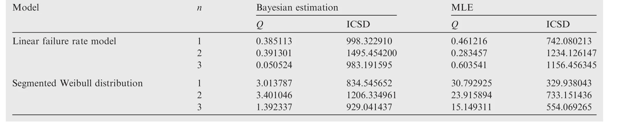
Table 4 Results of proximity sensors in leading-edge flap when μi= τi.

Table 5 Distribution parameters of proximity sensors in leading-edge flap when μi= τi.

Table 6 Results of proximity sensors in leading-edge flap when μi=0.

Fig.13 shows the best fitting of the failure rateh(t)of the proximity sensors in leading-edge flap.If all samples are not divided,the best distribution is a one-segment linear failure model,whose parameters are α=-0.057239,β=0.001525.From Fig.13,the error of non-segment fitting is very great,and even it is not a valid distribution.By comparison,segment distribution has an obvious advantage.

In addition,the following can be concluded from this example.(1)Usually,no matter what distribution samples follow,they are measured from perspective of the whole lifetime.However,after the samples are divided,the local property of the samples plays a more important role.The segmented distribution emphasizes the local characteristics of the samples,thus the expression of segmented distribution is often not the sameas that of non-segmented distribution.For instance,even if the samples follow Weibull distribution,they may no longer follow segmented Weibull distribution after segmentation.(2)Although the reliability function of segmented distribution is continuous,the segmented failure rate functionh(t)may be often discontinuous whether it is a linear failure rate mode or segmented Weibull distribution.

Table 7 Distribution parameters of proximity sensors in leading-edge flap when μi=0.

6.Conclusion and discussion

In this paper,twon-segment segmented reliability models are proposed,and then how to estimate parameters of these segmented reliability models by Bayesian estimation and MLE is discussed.Whatever in the simulation verification or in the application examples,the segmented distribution and its estimation methods have achieved good effects.Nevertheless,there are still some problems related to the segmented distribution,which deserve our further study.

(1)The unknown parameters in the segmented distribution are relatively too many,which makes the application of the segmented distribution become more difficult.Thus,concise segmented distribution should be discussed,which should be widely used in many fields,such as classification and clustering.

(2)Although the estimation methods for the segmented distribution are discussed in this paper,these methods are still not accurate enough in estimating μi, τi,so in future research,better estimation methods should be studied,especially some methods to accurately estimate μi,τi.

(3)The segmented function h(t)discussed in this article is usually discontinuous,which may be inconsistent with real circumstances.Although the reliability function is continuous,errors may still occur,so continuous segmented distribution should be discussed in the future.

(4)Only when there exist change-points in failure rate,the segmented distribution can take its advantage.Thus there is a problem of detecting change-points before estimation by the segmented distribution.In this paper,merely MLE is preliminarily discussed to test changepoints,which is not sufficient.In the future,methods to detect change-points should deserve a careful study,especially from the perspective of Bayesian method and likelihood ratio method.

(5)From the experiments in this paper,it’s concluded that precision of the Gibbs sampling method is not suff iciently high.In future research,it is necessary that the Gibbs sampling method should be modified to improve its accuracy.

Acknowledgements

This work was supported by the National Natural Science Foundation of China(Nos.60672164,60939003,61079013,60879001,90000871),the Special Project about Humanities and Social Sciences in Ministry of Education of China(No.16JDGC008),National Natural Science Funds and Civil Aviation Mutual Funds(Nos.U1533128 and U1233114),Study On Reusing Sketch User Interface Oriented Design Knowledge(No.16KJA520003),and Six Talent Peaks Project In Jiangsu Province(No.2016-XYDXXJS-088).

1.Zhao XL,Qian T,Mei G,Kwan C,Zane R,Walsh C,et al.Active health monitoring of an aircraft wing with an embedded piezoelectric sensor/actuator network:II.Wireless approaches.Smart Mater Struct2007;16(4):1218–25.

2.Wu B,Tian Z,Chen M.Condition-based maintenance optimization using neural network-based health condition prediction.Qual Reliab Eng Int2012;29(8):1151–63.

3.Bae SJ,Mun BM,Kim KY.Change-point detection in failure intensity:a case study with repairable artillery systems.Comp Indust Eng2013;64(1):11–8.

4.Toms JD,Lesperance ML.Piecewise regression:A tool for identifying ecological thresholds.Ecology2003;84(8):2034–41.

5.Atashgar K.Identification of the change point:an overview.Int J Adv Manuf Technol2013;64(9–12):1663–83.

6.Bae SJ,Yuan T,Ning SL,Kuo W.A Bayesian approach to modeling two-phase degradation using change-point regression.Reliab Eng Syst Safety2015;134:66–74.

7.Kvam PH.A change-point analysis for modeling incomplete burnin for light displays.IIE Trans2006;38:489–98.

8.Li YX,Qian LF,Zhang W.Estimation in a change-point hazard regression model with long-term survivors.Statist Probab Lett2013;83(7):1683–91.

9.He P,Kong G,Su Z.Estimating the survival functions for rightcensored and interval-censored data with piecewise constant hazard functions.Contemp Clin Trials2013;35(2):122–7.

10.Uhm D,Huffer FW,Park C.Additive risk model using piecewise constanthazard function.CommunStatist—SimulComput2011;40(9):1458–77.

11.Liu ZH,Qian LF.Changepoint estimation in a segmented linear regression via empirical likelihood.Commun Statist—Simul Comput2009;39(1):85–100.

12.Goodman MS,Li Y,Tiwari RC.Detecting multiple change points in piecewise constant hazard functions.J Appl Statist2011;38(11):2523–32.

13.Suresh RP.A test for constant hazard against a change-point alternative.Commun Statist—Theory Meth2012;41(9):1583–9.

14.Nosek K,Szkutnik Z.Change-point detection in a shape-restricted regression model.Statist:A J Theoret Appl Statist2013;48(3):641–56.

15.Chou K,Tang K.Burn-in time and estimation of change-point with Weibull-Exponential mixture distribution.Dec Sci1992;23(4):973–90.

16.Achcar JA,Loibel S.Constant hazard function models with a change point:A Bayesian analysis using Markov chain Monte Carlo methods.Biomet J1998;40(5):543–55.

17.Boukai B.Bayes sequential procedure for estimation and for determination of burn-in time in a hazard rate model with an unknown change point parameter.Seq Anal1987;6(1):37–53.

18.Patra K,Dey DK.A general class of change point and change curve modeling for life time data.Ann Inst Statist Math2002;54(3):517–30.

19.Igba J,Alemzadeh K,Anyanwu-Ebo I,Gibbons P,Friis J.A systems approach towards reliability-centred maintenance(RCM)of wind turbines.Proc Comp Sci2013;16(1):814–23.

20.Dehghanian P,Fotuhi-Firuzabad M,Aminifar F,Billinton R.A comprehensive scheme for reliability centered maintenance in power distribution systems—Part I:Methodology.IEEE Trans Power Deliv2013;28(2):761–70.

21.Li YX,Qian LF.Likelihood ratio test for a piecewise continuous Weibull model with an unknown change point.J Math Anal Appl2014;412(1):498–504.

22.Pandya M,Jani PN.Bayesian estimation of change point in inverse Weibull sequence.Commun Statist-Theory Meth2006;35(12):2223–37.

23.Zhang T,Xie M.On the upper truncated Weibull distribution and its reliability implications.Reliab Eng Syst Safety2011;96(1):194–200.

24.Sarhan AM,Apaloo J.Exponentiated modified Weibull extension distribution.Reliab Eng Syst Safety2013;112(4):137–44.

25.Maboudou-Tchao Edgard M,Hawkins Douglas M.Detection of multiple change-points in multivariate data.J Appl Statist2013;40(9):1979–95.

26.Hu Y,Zhao K,Lian H.Bayesian quantile regression for partially linear additive models.Statist Comput2015;25(3):651–68.

27.Alhamzawi R,Yu K.Conjugate priors and variable selection for Bayesian quantile regression.Comput Statist Data Anal2013;64(4):209–19.

28.Reich BJ,Smith LB.Bayesian quantile regression for censored data.Biometrics2013;69(3):651–60.

29.Nosek K.Schwarz information criterion based tests for a changepoint in regression models.Statist Papers2010;51(4):915–29.

30.Pan JM,Chen JH.U-statistic based modified information criterion for change point problems.Commun Statist—Theory Meth2008;37(17):2687–712.

31.Chen JH,Pan JM.Information criterion and change point problem for regular models.Ind J Statist2006;68(2):252–82.

32.Shen G,Ghosh JK.Developing a new BIC for detecting changepoints.J Statist Plan Inf2011;141(4):1436–47.

33.Ninomiya Y.Information criterion for Gaussian change-point model.Statist Probab Lett2005;72(3):237–47.

34.Hannart A,Naveau P.An improved Bayesian information criterion for multiple change-point models.Technomet A J Statist Phys Chem Eng Sci2012;54(3):256–68.

35.El-Gohary A,Alshamrani A,Al-Otaibi AN.The generalized Gompertz distribution.Appl Math Model2013;37(1–2):13–24.

36.Mazucheli J,Coelho-Barros EA,Achcar JA.Inferences for the change-point of the exponentiated Weibull hazard function.REVSTAT2012;10(3):309–22.

37.Xie M,Lai CD.Reliability analysis using an additive Weibull model with bathtub-shaped failure rate function.Reliab Eng Syst Safety1996;52(1):87–93.

38.Bebbington M,Lai CD,Wellington M,Zitikis R.The discrete additive Weibull distribution:A bathtub-shaped hazard for discontinuous failure data.Reliab Eng Syst Safety2012;106(5):37–44.

39.Jiang R.A new bathtub curve model with a finite support.Reliab Eng Syst Safety2013;119:44–51.

17 June 2015;revised 31 January 2016;accepted 18 October 2016

Available online 21 December 2016

Ⓒ2017 Production and hosting by Elsevier Ltd.on behalf of Chinese Society of Aeronautics and Astronautics.This is an open access article under the CC BY-NC-ND license(http://creativecommons.org/licenses/by-nc-nd/4.0/).

*Corresponding author.

E-mail addresses:li_huai_yuan@139.com(H.Li),rms@nuaa.edu.cn(H.Zuo),xj0601@nuaa.edu.cn(J.Xu).

Peer review under responsibility of Editorial Committee of CJA.