Temperature dependence of heat conduction coefficient in nanotube/nanowire networks∗

Kezhao Xiong(熊科诏)and Zonghua Liu(刘宗华)

Department of Physics,East China Normal University,Shanghai 200062,China

Temperature dependence of heat conduction coefficient in nanotube/nanowire networks∗

Kezhao Xiong(熊科诏)and Zonghua Liu(刘宗华)†

Department of Physics,East China Normal University,Shanghai 200062,China

Studies on heat conduction are so far mainly focused on regular systems such as the one-dimensional(1D)and two dimensional(2D)lattices where atoms are regularly connected and temperatures of atoms are homogeneously distributed. However,realistic systems such as the nanotube/nanowire networks are not regular but heterogeneously structured,and their heat conduction remains largely unknown.We present a model of quasi-physical networks to study heat conduction in such physical networks and focus on how the network structure influences the heat conduction coefficient κ.In this model, we for the first time consider each link as a 1D chain of atoms instead of a spring in the previous studies.We find that κ is different from link to link in the network,in contrast to the same constant in a regular 1D or 2D lattice.Moreover,for each specific link,we present a formula to show how κ depends on both its link length and the temperatures on its two ends. These findings show that the heat conduction in physical networks is not a straightforward extension of 1D and 2D lattices but seriously influenced by the network structure.

heat conduction,nanotube/nanowire,complex network,one-dimensional(1D)lattice

1.Introduction

Heat conduction in low dimensional systems such as onedimensional(1D)and two-dimensional(2D)lattices has been well studied,where one of the main focuses is the abnormal heat conduction.[1–3]These studies are based on the Fourier’s law

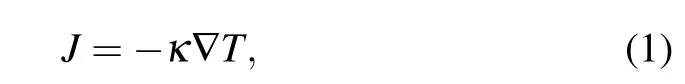
where the heat flux J is the amount of heat energy transported through the unit surface per unit time and T(x,t)is the local temperature.In the case of normal heat conduction,the coefficient κ is a constant,i.e.,size independent.However,in the case of abnormal heat conduction,the coefficient κ depends on the system size N,i.e.,κ∝Nα,[4–13]where α can be different constants in[0,1]for different models such as the FPU model,Frenkel–Kontorova(FK)model,φ4model,disordered harmonic chain,ding-a-ling model,Toda lattice,and Klein–Gordon lattice,depending on the mode coupling between the longitudinal modes and the transverse modes.

Compared to the intense studies of size dependence,only a few studies have been focused on the influence of the temperature on the coefficient κ.[14–16]These studies are focused on the cases of regular 1D and 2D lattices where the temperatures at different atoms are homogeneously distributed. However,in realistic situations such as the nanotube/nanowire networks,[17–21]the temperatures at different nodes are not homogeneously but heterogeneously distributed as the link lengths between any two connected nodes will not be the same. The heterogeneous distributed temperatures will seriously influence the heat fluxes on the individual links and then influence the total heat fluxes in the network.This prediction has been confirmed in an oversimplified network model where the links are simplified as springs.[22,23]

Then,an open question is how the structure of a real network,such as links being the nanotubes/nanowires,influences the heat conduction.More important is how the network structure influences the coefficient κ.The importance of this question can be understood from the following two aspects.Firstly, different links of the network are connected to different nodes with distinctive temperatures,indicating that they have different environments.Secondly,the temperatures at different nodes are substantially different from that of heat baths as the former is correlated to the dynamics of the network while the latter is independent of the network.In this sense,do we still have the formula κ∝Nαfor different links in the network or should we have a new formula for κ?

To figure out the answer,for convenience,we here present a model of quasi-physical networks in which each link is assumed to be a 1D chain with finite atoms,in contrast to the simplified springs in Ref.[22].Figure 1 shows its schematic diagram,where the yellow points with circles represent the nodes,the blue points denote the atoms on the links,the red and black points with circles represent the two source nodes contacting heat baths with high temperature Thand low temperature Tl,respectively,and nijdenotes the number of atoms on link lij.In this kind of network,the nodes’degrees are het-erogeneously distributed,such as ki=5 and kj=7 in Fig.1, in contrast to the constant degrees of ki=2 in 1D lattice and ki=4 in 2D lattice.More importantly,the link length nijis also not a constant as in 1D and 2D lattices but different for different links.When the network reaches its dynamical equilibrium or stationary state,the temperature at each node will be fixed.In this state,each individual link is connected to two nodes with fixed temperatures,which can be considered as a pair of heat sources with high and low temperatures,respectively.In this case,we see that different links of the network are in different environments of different local temperatures and thus may have different κ,indicating that the heat conduction in the network is fundamentally different from that in regular 1D and 2D lattices.Therefore,it is very important for us to understand how κ depends on the temperatures at the two ends of a link,except the size dependence,which is our motivation here.

Fig.1.(color online)Schematic figure of a nanotube/nanowire network model,where the yellow points with circles represent the nodes, the blue points denote the atoms on links,i0 and j0 represent the two heat source nodes contacting two thermostats with low temperature T l and high temperature T h,respectively,and nij represents the number of atoms between the two connected nodesiand j.

The paper is organized as follows.In Section 2,we focus on a variety of 1D chains with different lengths and temperatures and discuss how the heat conduction coefficient κ depends on the temperature,temperature difference,and chain lengths.In Section 3,we discuss both the heat conduction and the coefficient κ in physical networks,aiming to reveal the influence of the network structure on κ.In Section 4,we give a brief discussion and conclusions.

2.Heat conduction on a variety of 1D chains with different lengths and temperatures

To study how the network structure influences the coefficient κ,we first study the heat conduction on the individual links.For this purpose,we consider a 1D FPU-β chain of N coupled atoms with the two ends contacting thermal baths of higher temperature Thand lower temperature Tl,respectively.[1]We choose the thermal baths as the Nose– Hoover thermostat.[24]The chain has a Hamiltonian

where

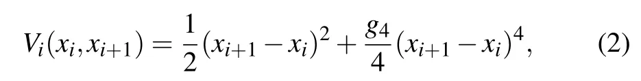
and xirepresents the displacement from the equilibrium position of the i-th atom.The motion of the atoms(i=2,3,...,N−1)satisfies the canonical equations

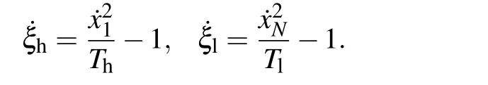
The dynamical equations for the heat baths are

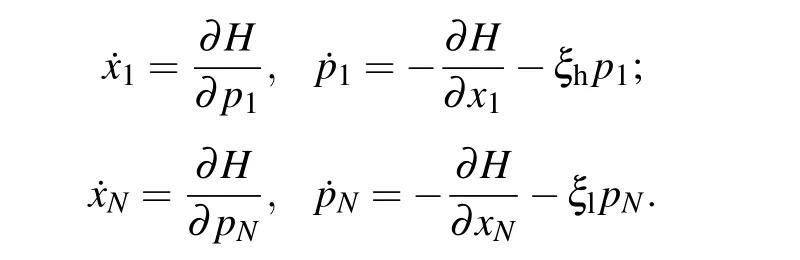
The dynamical equations for the first and the last atoms are

In this work,we let g4=0.1,which gives α=1/2,i.e.,

After the transient process,the chain will reach a stationary state.The local temperature at each atom can be defined

where〈···〉is the time average.When two neighboring atoms have different local temperatures,there will be a heat flux Jifrom the higher temperature to the lower temperature,which can be calculated by[1,27–29]

For a single chain,Jiwill be site independent.

In numerical simulations,we take Tl=3.0 and Th= 3.0+ΔT,where ΔT is the temperature difference between Thand Tl.Substituting κ∼Nαfor g4=0.1 into Eq.(1),we have 1/J∼N1−αwith α=0.4∼0.5.[26]To confirm this relationship,we first choose different sizes of N and let ΔT gradually increase from 0.2 to 0.8.Figure 2(a)shows the results.Then, we let ΔT gradually increase from 2.0 to 6.0.Figure 2(c) shows the results.From Figs.2(a)and 2(c),we see that all the lines are approximately straight with a common slope of 0.6 in(a)and 0.56 in(c),confirming 1/J∼N1−α.Furthermore, from Fig.2(a),it is also easy to notice that all the lines are not overlapped,reflecting the effects of Tland ΔT.To figure out the influence of ΔT,we fix both the size N and temperature Tland then check the dependence of flux J on ΔT,Figures 2(b) and 2(d)show the results for relatively small and large ΔT,respectively.We interestingly find that all the cases in Figs.2(b) and 2(d)can be approximately fitted by the straight lines with the same slope 0.92,implying J∼ΔT0.92.Then,an interesting question is what is the exact expression of κ.For simplicity, we assume

with α=0.5∼0.6.Substituting it into Eq.(1),we have

which gives

Thus,(1+γ)is nothing but the slope of the lines in Fig.2(b), which gives γ=−0.08.

To figure out the function f(Tl)in Eq.(5),we fix ΔT and N and gradually increase Tl.Figures 3(a)and 3(b)show the results for the cases of ΔT=1.5 and 0.75,respectively, where the squares,circles,and triangles represent the cases of N=36,64,and 100,respectively.All the results in Figs.3(a) and 3(b)show that f(Tl)is approximately dependent on Tlby a power lawwith η=−0.26 for ΔT=1.5 and η=−0.32 for ΔT=0.75,indicating that f(Tl)may be different for different ΔT.These results are not consistent with those of Ref.[14]where κ(T)scales differently in different temperature range,i.e.,it is 1/T for small T and T1/4for large T.As the value of g4=0.1 in our case is much smaller than that of g4=1.0 in Ref.[14],it is reasonable for our η=−0.26 or−0.32 to be in-between[−1,1/4]of Ref.[14].

Fig.2.(color online)Heat conduction in a chain with T l=3.0 and T h=3.0+ΔT.Panels(a)and(b)show the results of small ΔT:(a)1/J versus N,(b)J versus ΔT.Panels(c)and(d)show the results of large ΔT:(c)1/J versus N,(d)J versus ΔT.

Fig.3.(color online)J versus T l for fixed(a)ΔT=1.5 and(b)ΔT=0.75, where the squares,circles,and triangles represent the cases of N=36,64, and 100,respectively.

We conclude that the dependence of κ on the three factors of Tl,ΔT,and N can be approximately,expressed as

Equation(8)tells us that κ will not have the same value for different 1D chains as their three factors f(Tl),ΔT,and N are different in different conditions/environments.

3.Heat conduction and coefficient κ in quasiphysical networks

We here use Fig.1 as the model of real nanotube/nanowire networks and call it a quasi-physical network. Based on the above results,we understand that the heat conduction coefficient κ for a link lijdepends on three factors Ti, Ti–Tj,and nij.As the three factors are different from link to link in the network,κ will be different for different links.Even for those links with the same length nij,their κ will be different as the other two factors Tiand Ti–Tjare different.Therefore,the heat conduction in real networks will be fundamentally different from that in 1D and 2D lattices with a constant κ,thus it is not correct to apply the same κ to all the links in the network of Fig.1,[30]which makes the study of heat conduction in real networks more challenging.Moreover,it has been pointed out that there are thermal interface resistances at every node and their values depend sensitively on the site of the node and the coupling strength of each link.[23]In general, it is difficult to measure the thermal interface resistances for individual links,implying that it is almost impossible to make a theoretical study of heat conduction in real networks.Due to all these challenges,we here study the heat conduction in physical networks by numerical simulations.

In simulations,the model of physical networks of Fig.1 can be implemented as follows.Firstly,we construct a general network by the algorithm of Ref.[31],where a network in-between the scale-free and random networks can be produced by adjusting a parameter p.In detail,we take m0nodes as the initial nodes and then add one node with m links at each time step.The m links from the added node go to m existing nodes with probability Πi∼(1−p)ki+p, where kiis the degree of nodeiat that time and 0≤p≤1 is a parameter.The resulting network has an average degree〈k〉=2m for large N.Obviously,(1−p)kiin Πirepresents the preferential attachment and p in Πirepresents the random attachment.The resulting connectivity distribution will be a power-law P(k)∼k−γwith γ=3 for p=0,i.e.,the Barabasi–Albert scale-free network,[32]an exponential distribution P(k)∼e−k/mfor p=1,i.e.,the random network,and other complex networks in-between the random and scale-free networks for 0≤p≤1.We here let m0=3 and m=2,i.e.,〈k〉=4.

Secondly,for a fixed degree distribution P(k),the network topology can be still changed by adjusting the clustering coefficient of the network,C,which represents the possibility that two neighbors of a given node will also be neighbors,and can be calculated as follows:[32]

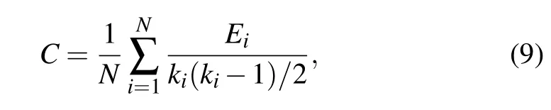
where kiis the degree of nodeiand Eiis the number of edges among the neighbors of node i.We here change the clustering coefficient by the Kim’s rewiring approach,[33]which has the advantage that the degree of each node will remain unchanged when we change its clustering coefficient.The algorithm of the rewiring approach can be stated as follows:we randomly choose two links,one connecting nodes A and B,and the other connecting nodes C and D.Then,we let each node change its partner and the original links A–B and C–D are altered to A–D and B–C.The link exchange trial is accepted only when the new network configuration has a higher clustering coefficient.

Thirdly,we let each link of the network be a 1D chain of atoms and each nodeiof the network be the cross atom of the kilinks of node i.In this sense,each atom on a link will have two neighbors and satisfy Eq.(2),while the atom at each nodeiwill have kineighbors and does not satisfy Eq.(2).We here let the atom at nodeisatisfy

where the sum is for all the nearest neighbors j of node i. Other dynamics of the node are the same as those of the atoms in a 1D chain.In detail,for a specific link lijbetween nodesiand j,we let it be a 1D chain of nijatoms,where nijis a random number from a uniform distribution and satisfies n1≤nij≤n2,i.e.,nij=n1+(n2−n1+1)×rand.We here let n1=3 and n2=11.It is clear that each atom on a link has only two nearest neighboring couplings while each atom at nodeihas kinearest neighboring couplings.We let Tirepresent the temperature of nodeiand Jijrepresent the heat flux of the link ij.

We let both the nodes and the atoms on the links be the same FPU-β atom.Their potentials satisfy Eqs.(10)and(2), respectively.We randomly choose two nodes i0and j0as the source nodes to contact two heat baths with temperatures Thand Tl,respectively,see Fig.1.We let Th=7 and Tl=3 in the following discussion.At node i0,the heat flux will be transmitted to other nodes through all the links of node i0.Near node j0,all the fluxes will gradually merge and finally go to node j0through the links of node j0,see the red arrows in Fig.1.Therefore,the heat flux from node i0to node j0depends partially on the structure of the network,such as the degree distribution and clustering coefficient.

For convenience,we here take the network size N=50 and the average links〈k〉=4 as it is time consuming for a larger network to reach the stationary state.After the transient process,the heat conduction on the network will reach a stationary state.The heat flux Jijat each link can be calculated by Eq.(4),while the total flux at a node will be zero, except the two source nodes i0and j0.The temperature at nodeican be obtained by Eq.(3).We denote the total heat flux of the network as the heat flux from node i0to node j0, Ji0→j0,which is the sum on all the paths from node i0to its neighbors or the sum on all the paths to node j0.By changing the network topology and the node pair(i0,j0),we can calculate other Ji0→j0.In this way,for each p,we randomly produce 50 networks with the same C and randomly choose one pair of nodes(i0,j0)for each produced network and then calculate their average J≡〈Ji0→j0〉.The squares in Fig.4(a) show the dependence of J on p for C=0.1.We see that J increases monotonously with p,indicating that the random network is in favor of energy diffusion.Then,we use the above rewiring approach to increase the clustering coefficient.Without rewiring,the clustering coefficient is C≈0.08.We now increase the clustering coefficient to C≈0.4 and recalculate the dependence of J on p.The circles in Fig.4(a)show the results.We see that its increase with p is similar to the case of C=0.1.

Fig.4.(color online)The heat fluxes J≡〈Ji0→j0〉versus p at stationary state with T h=7 and T l=3 For each p,the flux J is an average on 50 randomly produced networks with the same C.Panels(a)and(b)show the results of〈k〉=4 and 6,respectively.

Figure 5 shows the distribution of heat fluxes in one realization for a scale-free network with p=0 and C=0.1. The color of nodes represents its temperature where the red and black denote the highest and lowest temperatures,respectively,and the other colors in-between denote the temperatures in-between Thand Tl.We can see that these temperatures are heterogeneously distributed between Thand Tl.The arrows in Fig.5 show the directions of the heat fluxes and the width of the arrow between nodesiand j represents the strength of flux Jij.We see that the fluxes connected to the two heat source nodes are larger while the fluxes on the other links are relatively small,indicating that the flux from the source node with This firstly distributed to the network,then goes through different paths,and finally merges into the source node with Tl.

Fig.5.(color online)Distribution of heat fluxes in one realization for a scale-free network with p=0 and C=0.1,where the nodes 35 and 16 have been chosen as the heat source nodes with T h=7 and T l=3, respectively.

From Figs.4(a)and 5,we see that the total flux is seriously influenced by the network topology.For a fixed network structure,the heat fluxes are different from link to link. Then,an important question is how the network structure influences formula(6)of heat conduction.In other words,does formula(6)still work for the links in a network?To conveniently check it,we here focus on those links from a common node i,i.e.,the neighboring links lijfor j=1,2,...,ki.The reason for this choice is that these links have the common Tl, thus we need only to focus on the aspects of nijand ΔTijin Eq.(6).We here calculate the relationship betweenand ΔTijfor different j.Figure 6 shows the results for four typical nodesiin the random network with p=1,where(a) and(b)represent the cases of two typical nodes in the network with C=0.1,respectively,and(c)and(d)represent the cases of two typical nodes in the network with C=0.6,respectively. From each of the four typical cases in Fig.6,we see that the points are a little scattered.For conveniently investigating the relationship betweenand ΔTij,we draw a straight line for each case in Fig.6 to make the points be distributed around it.However,we find that the slopes of these straight lines are not the same but with the values of approximately 0.79,0.82,0.87,and 0.86 in Figs.6(a)–6(d),respectively,indicating that we do not have a common scaling exponent γ as in Eq.(6).We have also observed the same results for the scale-free network with p=0.These results tell us that κ in the links of the network is significantly different from that in a single 1D chain.Therefore,the heat conduction in real networks is seriously influenced by the network structure,indicating the significant difference to the regular 1D and 2D lattices.

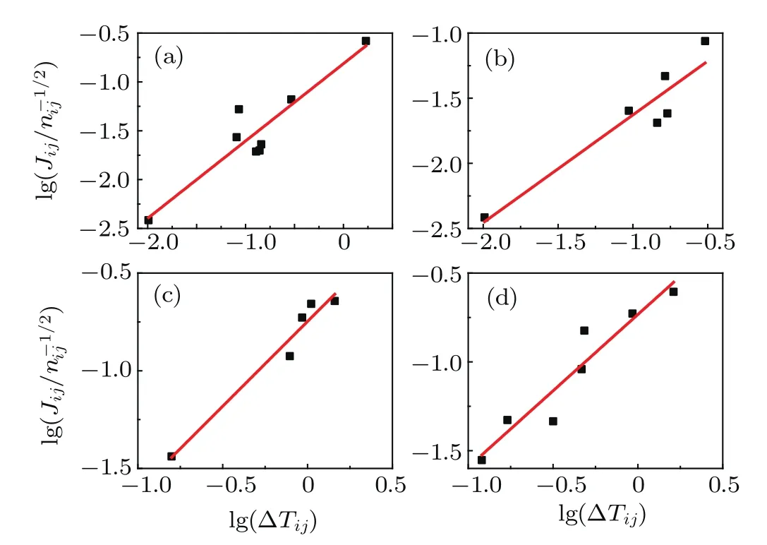
Fig.6.(color online)Dependence ofon ΔTij for a fixediand its different neighbors j where the network is chosen as the random network with p=1 and the straight lines are from the least square method. Panels(a)and(b)show the results of two typical nodes in the network with C=0.1,and panels(c)and(d)show the results of two typical nodes in the network with C=0.6.

Finally,we discuss the influence of the averaged degree〈k〉.Our numerical simulations show that〈k〉seriously influ-ences the total heat flux J in the network.Figure 4(b)shows the result for〈k〉=6.Comparing Fig.4(a)with Fig.4(b), we see that the flux J in(b)is much smaller than that in(a), confirming the topology influence again.

4.Discussion and conclusion

Generally,one may think that a nanotube/nanowire network consists of individual links and thus its heat conduction may be similar to that in 1D chain.But the results obtained here show that the heat conduction in a physical network is significantly different from that in 1D and 2D lattices.The coefficient κ depends on both the network topology and the temperature distribution,except the length of the chain,which is in contrast to the 1D and 2D lattices.This difference mainly comes from the fact that the temperatures at different nodes are correlated with each other and thus cannot be treated as the heat baths in 1D chain.

We have to point out that this quasi-physical network model is still far away from the realistic networks of nanotubes.That is,many key factors of the realistic networks are not considered,thus this model is not a model of real nanotube/nanowire networks but only the one going a substantial step toward the real ones.For example,for nanotubes of length around 100˚A,the thermal conductivity may become saturated to its size-independent value.In this way,the size-dependence only appears for very short nanotubes,probably shorter than commonly fabricated and applied ones.It is very difficult to make link lengths of 3 to 11 atoms in lab.The similar problem may also come from the phonon mean free path.Although these lack correspondence to real nanotubes,the model does reveal some interesting nonlinear effects such as the nonlinear response on both ΔTijand Tl.On the other hand,this model also raises some interesting questions for future studies,such as the relationship between the link lengths and the mean free path of phonons.

In summary,we have studied the heat conduction in quasi-physical networks and paid attention to the dependence of heat conduction κ on both the sizes of the links and the temperatures of the nodes.The constructed network is close to the real nanotube/nanowire networks as its links are composed of 1D chains of atoms.The study is finished by two steps.In step one,we focus on the case of a single link and pay attention to the influence of temperature on heat conduction.We find that for fixed heat baths of low temperature,the coefficient of heat conduction κ is inversely proportional to the temperature difference between the two heat baths,while for fixed temperature difference,κ is inversely proportional to the low temperature.In step two,we construct a quasi-physical network model to study heat conduction in realistic networks.We find that the dependence of κ on temperatures is significantly different from that in the single 1D chain.More importantly,the values of κ are different from link to link in the network and can be seriously influenced by the network structure.

[1]Lepri S,Livi R and Politi A 2003 Phys.Rep.377 1

[2]Li N B,Ren J,Wang L,Zhang G,Hanggi P and Li B W 2012 Rev.Mod. Phys.84 1045

[3]Dhar A 2008 Advances in Physics 57 457

[4]Lepri S 1998 Phys.Rev.E 58 7165

[5]Pereverzev A 2003 Phys.Rev.E 68 056124

[6]Narayan O and Ramaswamy S 2002 Phys.Rev.Lett.89 200601

[7]Payton D N,III and Visscher W M 1967 Phys.Rev.156 1032

[8]Li B W,Casati G and Wang J 2003 Phys.Rev.E 67 021204

[9]Kaburaki H and Machida M 1993 Phys.Lett.A 181 85

[10]Dhar A 2001 Phys.Rev.Lett.86 3554

[11]Rieder Z,Lebowitz J L and Lieb E J 1967 Math.Phys.8 1073

[12]Savin A V and Gendelman O V 2003 Phys.Rev.E 67 041205

[13]Liu Z H and Li B W 2008 J.Phys.Soc.Jpn.77 074003

[14]Li N B and Li B 2007 Europhys.Lett.78 34001

[15]Aoki K and Kusnezov D 2001 Phys.Rev.Lett.86 4029

[16]Zolotarevskiy V,Savin A V and Gendelman O V 2015 Phys.Rev.E 91 032127

[17]Liu S,Xu X F,Xie R G,Zhang G and Li B W 2012 Eur.Phys.J.B 85 337

[18]Li N B,Li B W and Flach S 2010 Phys.Rev.Lett.105 054102

[19]Stadermann M 2004 Phys.Rev.B 69 201402

[20]Skakalova V,Kaiser A B,Woo Y S and Roth S 2006 Phys.Rev.B 74 085403

[21]Xu H,Zhang S and Anlage S M 2008 Phys.Rev.B 77 075418

[22]Liu Z H,Wu X,Yang H J,Gupte N and Li B W 2010 New J.Phys.12 023016

[23]Liu Z H and Li B W 2007 Phys.Rev.E 76 051118

[24]Nose S 1984 J.Chem.Phys.81 511

[25]Hoover W G 1985 Phys.Rev.A 31 1695

[26]Lepri S,Livi R and Politi A 1997 Phys.Rev.Lett.78 1896

[27]Hu B B,Li B W and Zhao H 1998 Phys.Rev.E 57 2992

[28]Hu B B,Li B W and Zhao H 2000 Phys.Rev.E 61 3828

[29]Li B W,Wang L and Casati G 2004 Phys.Rev.Lett.93 184301

[30]Xiong Kezhao,Li Baowen and Liu Zonghua 2017 unpublished

[31]Liu Z H,Lai Y C,Ye N and Dasgupta P 2002 Phys.Lett.A 303 337

[32]Albert R and Barabasi A 2002 Rev.Mod.Phys.74 47

[33]Kim B J 2004 Phys.Rev.E 69 045101

22 March 2017;revised manuscript

4 June 2017;published online 18 July 2017)

10.1088/1674-1056/26/9/098904

∗Project supported by the National Natural Science Foundation of China(Grant Nos.11135001 and 11375066)and the National Basic Research Program of China(Grant No.2013CB834100).

†Corresponding author.E-mail:zhliu@phy.ecnu.edu.cn

©2017 Chinese Physical Society and IOP Publishing Ltd http://iopscience.iop.org/cpb http://cpb.iphy.ac.cn