Reconstructing the Potential Function in a Formulation of Quantum Mechanics Based on Orthogonal Polynomials

A.D.Alhaidari

Saudi Center for Theoretical Physics,P.O.Box 32741,Jeddah 21438,Saudi Arabia

1 Introduction

Recently,we introduced a formulation of quantum mechanics without the need to specify a potential function.[1−3]This was done under the assumption that there are quantum systems that could be described analytically but not their corresponding potential functions.The success of this formulation implies that the class of exactly solvable problems is larger than the well-known class in the conventional formulation of quantum mechanics(see,for example,Ref.[4]for the conventional class of solvable potential functions).In the new formulation,the role of the potential function is taken up by orthogonal polynomials in the energy as expansion coefficients of the wavefunction in a complete set of square-integrable basis functions in con figuration space.Speci fically,we write the total wavefunction as Ψ(t,x)=e−iEtψ(E,x),whereEis the energy of the system in the atomic units ħ=m=1 and[1−3]

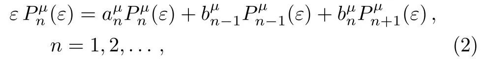
wherePµ0(ε)=1,Pµ1(ε)=αε+βand{aµn,bµn}are the recursion coefficients withbµn/=0 for alln.Ifα=1/bµ0and

whereτandξare real positive constants that depend on the particular polynomial.Aµ(ε)is the scattering amplitude andδµ(ε)is the phase shift.Bound states,if they exist,occur at(in finite or finite)energies that make the scattering amplitude vanish.That is,them-th bound state occurs at an energyEm=E(εm)such thatAµ(εm)=0 and the corresponding bound state is written as

where{Qµn(εm)}are the discrete version of the polynomials{Pµn(ε)}andωµ(εm)is the associated discrete weight function.In the absence of a potential function,the physical properties of the system are deduced from the properties of the associated orthogonal polynomials.Such properties include the shape of the weight function,nature of the generating function,distribution and density of the polynomial zeros,recursion relation,asymptotics,differential or difference equations,etc.

To establish a connection with the standard formulation of quantum mechanics,we try here to develop a procedure for reconstructing the potential function in the new formulation.There is no a priori guarantee that such a procedure will always yield an analytic potential function.Nonetheless,these results should be interesting especially if the derived potentials are associated with systems that do not belong to the conventional class of integrable systems in standard quantum mechanics.Examples of such systems were introduced in Refs.[1–3]where the energy polynomials are the Meixner–Pollaczek,continuous dual Hahn and Wilson polynomials in addition to their discrete versions of the Meixner,dual Hahn and Racah polynomials,respectively.It is,therefore,pressing to develop a procedure for reconstructing these new kind of non-conventional potential functions because of their possible physical applications.Many such applications could be found in atomic,molecular,chemical,optical,nuclear,and thermal physics.Recent example of the latter could be found in Refs.[5–8].Most of such applications are built on the con figuration space representation of the potential function.Thus,we need to develop a method of producing such representations starting from the orthogonal polynomials and basis elements.

The paper is organized as follows.In Sec.2,we outline the procedure of how to obtain the matrix elements of the potential in the chosen basis set{φn(x)}.Then,in Sec.3,we present four methods of how to construct the potential function numerically using knowledge of only its matrix elements and the basis set in which they are computed.In Sec.4,we test the procedure by applying it first on systems with known potential functions then in Sec.5 we give examples where we recover potentials that do not belong to the known class of exactly solvable problems in standard quantum mechanics.Some of these potentials are recovered analytically while others can only be reconstructed numerically.Mandating the correspondence(i.e.,demanding the existence of an analytic potential function)places a severe restriction on the kinematics of such problems.

2 The Potential Matrix Elements

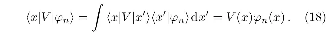
The first step is to calculate the matrix elements of the Hamiltonian operatorH. Now,the explicit construction of the total wavefunction of the system as Ψ(t,x)=e−iEt/ħψ(E,x)means thatHΨ =iħ(∂/∂t)Ψ =EΨ.Therefore,writing the wave equation asH|ψ〉=equation

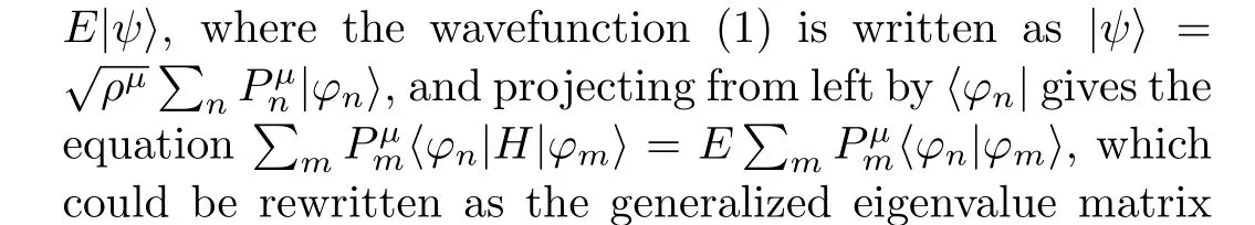
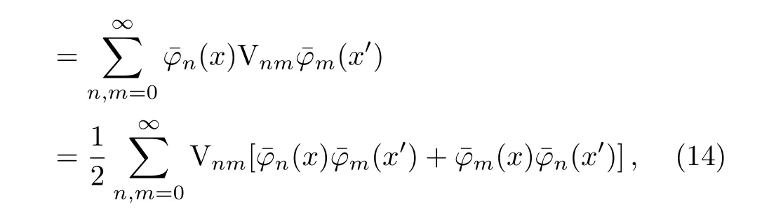
where H is the matrix representation of the Hamiltonian operator in the basis{φn}and Ω is the overlap matrix of the basis elements,Ωn,m=〈φn|φm〉(i.e.,matrix representation of the identity).On the other hand,the three-term recursion relation(2)could be rewritten in matrix form as Σ|P〉=ε|P〉,where Σ is the tridiagonal symmetric matrix obtained from Eq.(2)as

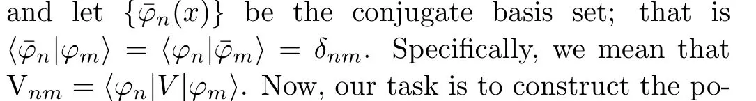
Therefore,the matrix wave equation H|P〉=EΩ|P〉must be equivalent to and should yield the three-term recursion relation Σ|P〉=ε|P〉.This implies that the wave operator matrix J=H−EΩ is“equivalent”to the matrix Σ−εin the space of the energy polynomials{Pµn}.For example,the matrix J should be tridiagonal and symmetric.This requirement places a restriction on the physical systems vis-`a-vis realization of the potential functions that are needed to establish a correspondence with the standard formulation.It should be noted that “equivalence”here means that the two tridiagonal matrices,H−EΩ and Σ−ε,are related via a similarity transformation.In this work,we use a notation whereby the matrix representation of the physical operators like the HamiltonianHand the potentialVare designated by non-italic capital letters(e.g.,H and V).

In standard quantum mechanics,the HamiltonianHis the sum of the kinetic energy operatorTand the potential functionV.Thus,V=H−Tand to obtain the matrix representation of the potential in the basis{φn}we need to compute the matrix elements of the kinetic energy in this basis.Now,Tis usually a well-known differential operator in con figuration space.For example,in one dimension with coordinatex,T=−(1/2)(d2/dx2)and in three dimensions with spherical symmetry and radial coordinater,T=−(1/2)(d2/dr2)+ℓ(ℓ+1)/2r2,whereℓis the angular momentum quantum number.Therefore,the action ofTon the given basis elements{φn}could be derived and its matrix representation T depends only on the choice of basis.The matrix wave operator becomes J=V+T−EΩ,which is required to be tridiagonal since the matrix wave equation J|P〉=0 should be equivalent to and should yield the three-term recursion relation(Σ−ε)|P〉=0.Now,ifΩ is non-tridiagonal(i.e.,the basis elements are neither orthogonal nor tri-thogonal),then the kinetic energy matrix T must have corresponding energy-dependent components to cancel those out.This cannot be required of the potential matrix V since the potential is assumed to be energy independent.If after that,the matrix T still has some non-tridiagonal components left over then those must be eliminated by counter components in V so that the net wave operator matrix J becomes tridiagonal.Therefore,establishing a correspondence of our formulation with the standard potential quantum mechanics places a severe restriction on the choice of basis{φn}and potential functions to only those that result in a tridiagonal matrix representation for the wave operator J=V+T−EΩ.

As an illustration of how to obtain the kinetic energy matrix,let us consider the following square integrable ba-sis elements in three dimensions with spherical symmetry

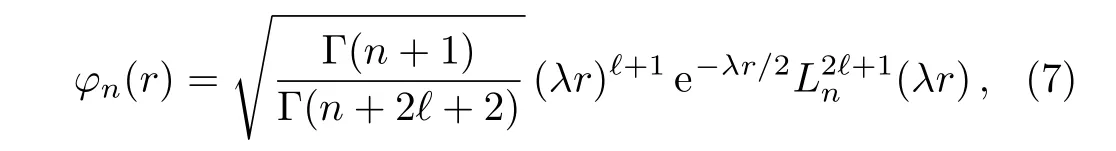
whereLνn(z)is the Laguerre polynomial of degreeninzandλ−1is a length scale parameter.Using the recursion relation and orthogonality of the Laguerre polynomials,we obtain

Moreover,the use of the differential equation of the Laguerre polynomial as well as its recursion relation and orthogonality we obtain

Therefore,the two matrices T and Ω are compatible with the correspondence procedure since they are tridiagonal.On the other hand,let us consider the following orthonormal set of elements as basis functions in one dimension

whereHn(z)is the Hermite polynomial of degreeninz.Using the differential equation of the Hermite polynomial,we obtain

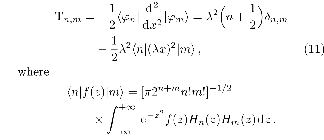
Therefore,the recursion relation of the Hermite polynomial and its orthogonality property show that the last term in Eq.(11)will produce non-tridiagonal components.In fact,this matrix component is penta-diagonal.Hence,it must be eliminated by the corresponding term+(1/2)λ4x2in the potential function,which is a harmonic oscillator potential term.This makes the sought after potential function equal toV(x)=(1/2)λ4x2+˜V(x)and turns our task into the construction of the potential component˜V(x)associated with the componentλ2(n+(1/2))δn,mof the kinetic energy matrix.On the other hand,using the recursion relation of the Hermite polynomial and its orthogonality property in Eq.(11)we obtain

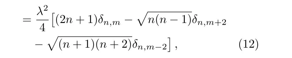
which is tridiagonal in function space with only odd or only even indices.That is,if the 1D problem conserves parity,then we can split function space into two disconnected subspaces(one odd and the other even)and T2n,2mis tridiagonal and so is T2n+1,2m+1.

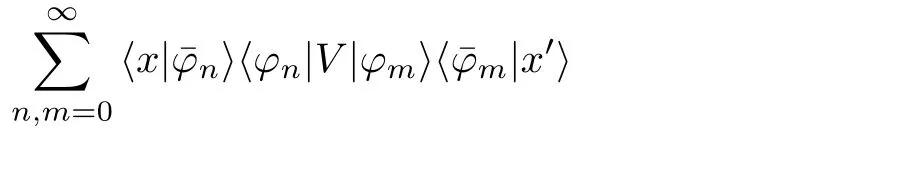
Our task now is to use knowledge of the matrix elements of the potential,which is obtained as Vn,m=Hn,m−Tn,m,and the basis in which they are computed to derive a realization of the potential function in con figuration space.Sometimes,we can recover the potential function analytically.However,in general reconstruction of the potential function from its matrix elements and the basis can only be done numerically.To achieve the latter,we present in the following section four alternative methods with different accuracy and range of applicability.Usually,the potential matrix obtained is finite in size.Thus,the derived potential function is an approximation that should improve with an increase in the size of the potential matrix.We will demonstrate this by descriptive examples where the potential function is known a priori.

3 The Potential Function

3.1 First Method

LetVdenote the quantum mechanical Hermitian operator that stands for the real potential energy.Then using Dirac notation,we can write

Therefore,we can write the approximation

3.2 Second Method

Of course,this is an approximation which is valid for finite values ofNsince the denominator blows up in the limit

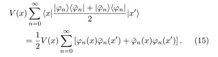
Using the completeness of(or the identity in)con figuration space,∫|x′〉〈x′|dx′=1,and Eq.(13)we can write

The completeness of the basis enables us to write the left side of this equation as

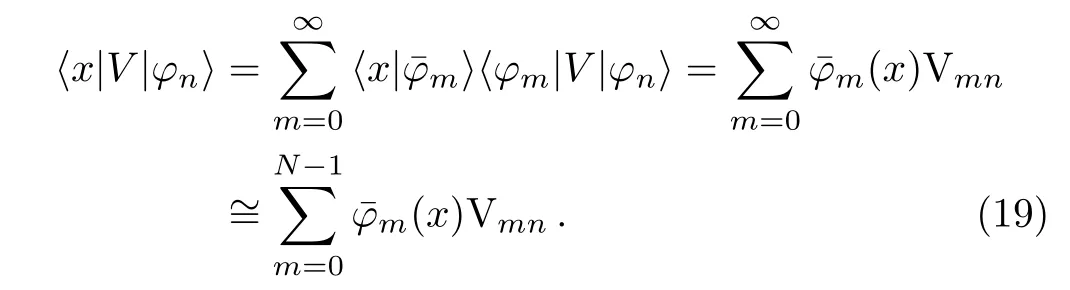
These two equations give

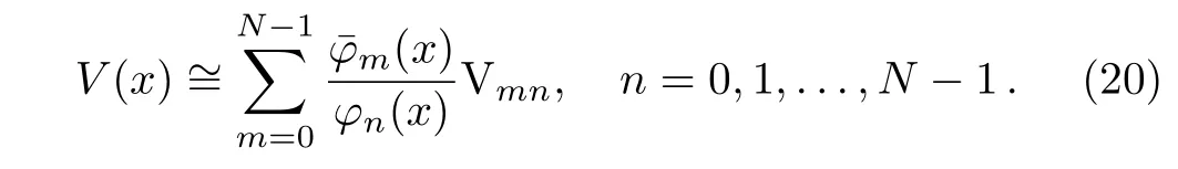
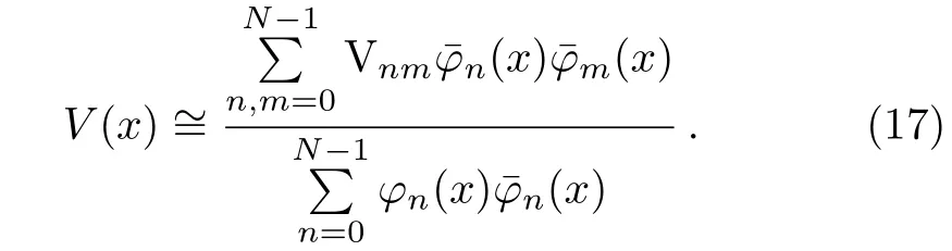
Therefore,we need the information in only one column of the potential matrix(or one row,since Vmn=Vnm)to determineV(x).In particular,if we choosen=0,we obtain

When comparing this method with the other three,we should take into consideration that this method uses onlyNelements of the potential matrix while the others use(1/2)N(N+1)elements.

3.3 Third Method

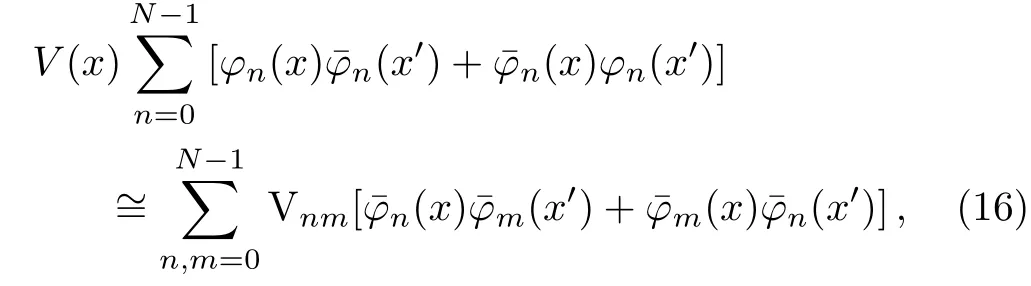
Completeness of the basis enables us to integrate Eq.(13)overx′as follows

3.4 Fourth Method

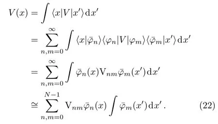
Fig.1 The solid thick curve is the potential function as recovered by the four methods using a basis size of 20.The thin curve with empty circles is the exact potential function,V(r)=5r2e−r.The basis used is that of Eq.(7)withℓ=1,λ=7 and the potential matrix elements are calculated using the Gauss quadrature associated with the Laguerre polynomials.The designation(3.n)means that the sub- figure was obtained using the n-th method introduced in section(3.n).

To test the above four methods,we select a priori the radial potential functionV(r)=5r2e−rin 3D and compute its matrix elements in the 3D basis of Eq.(7)withℓ=1 andλ=7 using the Gauss quadrature associated with the Laguerre polynomials.Then,we reconstruct the potential function using only these matrix elements and the basis as described above.Figure 1,shows that the third and fourth methods produce the best result.To make a stringent test of the third and fourth methods,we choose another nonanalytic potential function.Specifically,we consider the piece-wise linear potential function

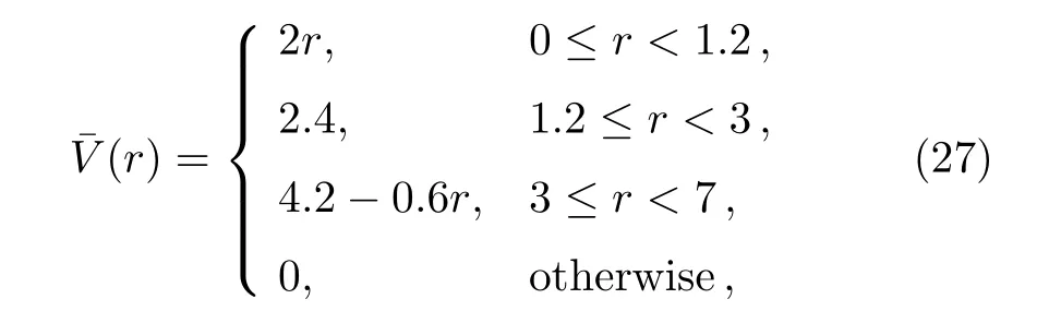
which is constructed to trace the functionV(r)=5r2e−r.Figure 2 is a plot of the two potential functions:V(r)and its nonanalytic version¯V(r).Figure 3 shows that the third method is superior to the fourth and illustrates the accuracy of the result with an increase in the size of the potential matrix.This may lead to the wrong conclusion that we should use only the third method in our study.However,in some cases(as will be demonstrated below)the other methods can produce superior results.Consequently,we will keep using all four methods in subsequent investigations.

In the following two sections,we use the procedure outlined in Sec.2 above to compute the matrix elements of the potential associated with a given system in our formulation of quantum mechanics.Then if the potential function could not be reconstructed analytically from these matrix elements and the basis,then we use one or more of the four methods to obtain an approximate graphical representation of the potential function.To demonstrate reliability and accuracy of the procedure,we start in the following section with two systems that have corresponding ones in the standard formulation of quantum mechanics with well-known potential functions.Thereafter in Sec.5,we present our original findings where we reconstruct the potential function of exactly solvable problems in our formulation none of which belong to the well-known class of exactly solvable problems in the conventional formulation of quantum mechanics.

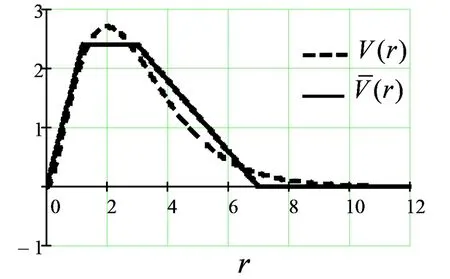
Fig.2 The dashed trace is the potential functions V(r)=5r2e−rwhereas the solid trace is its nonanalytic version¯V(r)de fined by Eq.(27).

Fig.3The left(right)plots are the results of recovering the nonanalytic potential¯V(r)using the third(fourth)method.The size of the basis are 10(top),20(middle)and 32(bottom).The designation(3.n)means that the sub- figure was obtained using the n-th method introduced in section(3.n).

4 Establishing the Correspondence:Conventional Problems

4.1 The Three-Dimensional Coulomb Problem

This problem was treated using our reformulation o

f quantum mechanics in Subsec.IV.A of Ref.[2].The energy polynomial that enters in Eq.(1)is the twonomials satisfy the symmetric three-term recursion relation shown as Eq.(B4)in the same Appendix.A proper basis for this problem is the one given by Eq.(7).Comparing the asymptotics of this polynomial,which is given by formula(B6),to the general formula(3)shows that the scattering phase shift(moduloπ/2)is

In standard quantum mechanics,this scattering phase shift is associated with the 3D Coulomb potentialVC(r)=−Z/r,whereZis the electric charge.Nonetheless,we will use the correspondence procedure outlined above to establish this fact.Substituting the physical parameters in the three-term recursion relation(B4),we obtain

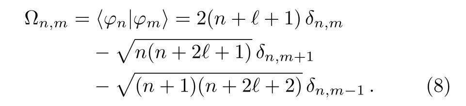
We rewrite this as the wave equation H|P〉=EΩ|P〉,where Ω is calculated using the basis(7)and given by Eq.(8).Thus,we obtain the following matrix elements of the Hamiltonian

Finally,the matrix representation of the potential function in the basis(7)are obtained as V=H−T,where the kinetic energy matrix T is given by Eq.(9).As a result,we obtain in fact a simple exact expression for the matrix elements of the potential in the appropriate basis(7)as Vn,m=−λZδn,m.Using these and the basis(7)with¯φn(r)=(λr)−1φn(r),we obtain an approximation of the potential function using the four methods given in the previous section.In this case,and for this potential,all methods except the third produce an exact match with the Coulomb potentialVC(r)for any basis sizeN.Nonetheless,we give in Fig.4 the result obtained by the third method that improves with increasingN.It is interesting to note that the simple identity matrix representationδn,min the basis(7)is obtained as matrix elements of the function(λr)−1in the basis(7).That is,〈φn|(λr)−1|φm〉=δn,mgiving the analytic realization of the potential as−Z/r.

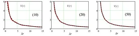
Fig.4 The red solid trace is the result of calculating the Coulomb potential using the third method as compared to the exact potential in dotted blue trace.We took Z=2,ℓ=1,and λ =3.The three parts of the figure correspond to basis size:10,20,50.

4.2 The One-Dimensional Morse Problem

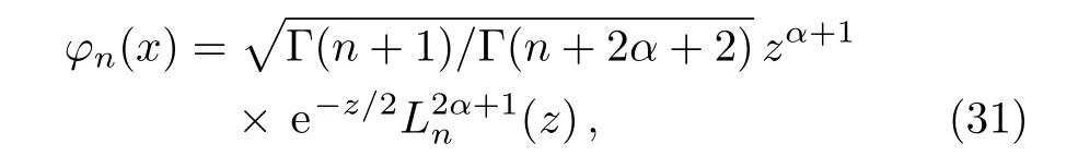
wherez=eλxwith−∞＜x＜+∞and we require thatα＞−1.From the asymptotics of the continuous dual Hahn polynomial,which is given by Eq.(B13),we obtain the scattering phase shift as

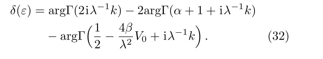
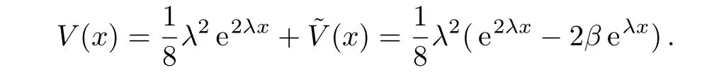
In standard quantum mechanics,this scattering phase shift is associated with the 1D Morse potentialVM(x)=V0(e2λx−2βeλx).[10]Substituting the physical quantities in the three-term recursion relation(B11)we obtain the matrix equationE|P〉=(λ2/2)Σ|P〉,where the matrix elements of Σ is obtained as

On the other hand,the matrix wave equation(5)could be rewritten asE|P〉= Ω−1H|P〉=H|P〉since Ωn,m=〈φn|φm〉=δn,m.Hence,we conclude that the Hamiltonian matrix is H=(λ2/2)Σ.Finally,we obtain the matrix elements of the potential function in the basis(31)as V=H−T,where the elements of the matrix T are Tn,m=−(1/2)〈φn|(d2/dx2)|φm〉.Using d/dx=λz(d/dz)and the differential equation of the Laguerre polynomial together with its differential property,

The recursion relation of the Laguerre polynomials and their orthogonality show that the third term on the right side of Eq.(34)produces non-tridiagonal matrix elements.Thus,the potential function must contain a counter term to cancel it so that the non-tridiagonal matrix component be eliminated.That is,the potential function must contain the term+(1/8)λ2z2=(1/8)λ2e2λxgivingV(x)=(1/8)λ2e2λx+˜V(x).Thus,our search will then be for the component˜V(x)which is associated with the kinetic energy matrix(34)without the(1/4)〈n|z2|m〉term and which reads as follows

Using the Hamiltonian matrix from(33)and this kinetic energy matrix we obtain the following potential matrix corresponding to˜V(x)as(λ2/2)Σ−˜T giving

Now,using these matrix elements and the basis(31),we calculate the potential function component˜V(x).For this problem,the second method produces an exact match toVM(x)withV0=(1/8)λ2for any basis sizeN.The third method produces only oscillations that diverge with increasingN.Figure 5 shows the results of the first and fourth methods.On the other hand,we can show that the three terms inside the square brackets of the potential matrix(37)is obtained as〈φn|z|φm〉.Thus,we can write the exact realization˜V(x)=(λ2/4)(2µ−1)z=−2βV0eλxgiving the full potential function as

With these two illustrative examples,we demonstrated that:

•Our strategy for establishing the correspondence between our reformulation of quantum mechanics without a potential and the standard formulation works since we were able to reconstruct the potential function either analytically or numerically.

•All four numerical methods established above should be used in the process since their accuracy differ from one problem to the other.

So far,we established correspondence between our formulation of quantum mechanics without a potential and the standard formulation by reconstructing the potential functions associated with well-known sample problems that included the Coulomb and Morse potentials.Next,we reconstruct the potential functions for problems that do not belong to the conventional class of exactly solvable potentials.We divide the problems into two classes.One where we could reconstruct the potential function analytically whereas for the other we could do that only numerically.

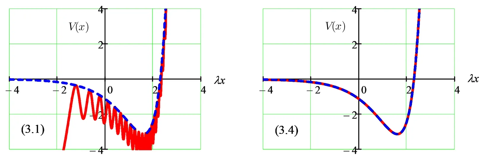
Fig.5 The red solid trace is the result of calculating the Morse potential using the first and fourth methods as compared to the exact potential in dotted blue trace.We took β =5,λ =1,V0= λ2/8 and α =3.The basis size was taken 100 for the first method and 10 for the fourth method.The designation(3.n)means that the sub- figure was obtained using the n-th method introduced in section(3.n).

5 Establishing the Correspondence:Nonconventional Problems

5.1 Analytic Realization of the Potential

In this subsection,we give two examples to demonstrate how to recover the potential function analytically.We take the following square integrable Jacobi basis

whereP(µ,ν)n(z)is the Jacobi polynomial of degreeninzand the real parameters are such thatα＞0 andν＞−1.The coordinate transformationz(x)is such that−1≤z≤+1 and the normalization constant is

We consider two cases in the following two subsections.Both do not belong to the conventional class of exactly solvable problems in the standard formulation of quantum mechanics.However,we will be able to give in both cases an analytic reconstruction of the potential function.

5.1.1Sinusoidal Potential Box

We takez(x)=sin(λx)where−π/2λ≤x≤+π/2λ.Then,we can show that if 2α=ν+(1/2)then Ω becomes diagonal(i.e.,the basis elements(38)are orthogonal)and the kinetic energy matrix reads as follows

The recursion relation of the Jacobi polynomials and their orthogonality show that the second term on the right side of Eq.(39)produces non-tridiagonal matrix elements.Thus,the potential function must contain a counter term to cancel it so that we end up with only a tridiagonal matrix.That is,the potential function must contain the term

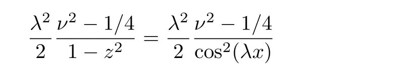
givingV(x)=(V2/cos2(λx))+˜V(x)with the basis parameterν2=(1/4)+2V2/λ2requiring the potential parameterV2≥−λ2/8.Thus,our search will be for the component ˜V(x)which is associated with the kinetic energy matrix

Now,since Ω and˜T are diagonal then to maintain the tridiagonal structure of the wave operator we require that the matrix elements〈φn|˜V(x)|φm〉must be at most tridiagonal.Noting that

then〈φn|˜V(x)|φm〉=〈n|˜V(x)|m〉and the recursion relation of the Jacobi polynomial and its orthogonality dictate that˜V(x)be a linear function inz.That is,˜V(x)=V0+V1sin(λx)and then the total potential function becomes

whereν2=(1/4)+(2V2/λ2).Figure 6 is a plot of this potential obtained by varying one parameter while keeping the other two fixed.The first and last term of the potential correspond to well-known and exactly solvable potentials in standard quantum mechanics.They constitute a special case of either the trigonometric Poschl–Teller potential or the trigonometric Scarf potential.Nonetheless,withV1/=0 this potential,which is exactly solvable in our reformulation,does not belong to the conventional class of exactly solvable problems.The pureV1potential term represents a potential box with sinusoidal bottom,which is not known to have an exact solution in standard quantum mechanics.[11]Using the recursion relation of the Jacobi polynomial and its orthogonality,we obtain the following matrix elements of the potential function˜V(x)

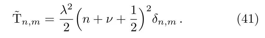
Adding to this the corresponding kinetic energy matrix˜T of Eq.(41)we obtain the Hamiltonian matrix.WithΩn,m=〈φn|φm〉=δn,m,the wave equation(5),H|P〉=EΩ|P〉,results in the following symmetric three-term recursion relation for the corresponding energy polynomial

whereε=2E/λ2andui=2Vi/λ2.This energy polynomial and its corresponding weight function are those that enter in the expansion series of the wavefunction(1)for this problem.

Fig.6 Plot of the potential(42)obtained by varying the parameter V1while keeping the other two fixed at V0=0 and V2= λ2.We took λ =1 and varied V1from 0(top curve)to 5(bottom curve)in units of λ2.The x-axis is measured in units of π/2λ.

5.1.2Hyperbolic Potential Pulse

Therefore,to cancel the non-tridiagonal terms in Ω,we require thatν2=−2E/λ2making the basis parameterνenergy dependent and dictating that an exact solution is obtained only for negative energy.Moreover,we obtain the following wave operator matrix

Therefore,the tridiagonal requirement of this matrix and the recursion relation of the Jacobi polynomial and its orthogonality dictate thatV(x)/(1−z2)=V0+V1zgiving the following potential function

WithV1/=0,this potential does not belong to the conventional class of exactly solvable problems.Figure 7 is a plot of this potential obtained by varyingV0while keepingV1fixed.Since the solution is valid for negative energy then the ratio|V0/V1|must be less than one.[12]Finally,the wave operator matrix(46)becomes

whereui=2Vi/λ2.Note that the energy is embedded in the parameterν.The matrix wave equation J|P〉=0 gives the following three-term recursion relation for the corresponding energy polynomials that enter as expansion coefficients of the wave function(1)

Fig.7 Plot of the potential(47)obtained by varying the parameter V0while keeping the V1 fixed at V1=1.5λ2.We took λ =1 and varied V0from −1(bottom curve)to+1(top curve)in units of λ2.

5.2 Numerical Realization of the Potential

In this subsection,we present two examples where we will not be able to recover the potential function analytically.Nonetheless,we can still reconstruct it numerically by using any of the four techniques established in Sec.3 above.Here,we consider a physical system on the positive real line where the basis elements are chosen as follows

wherez(x)=2tanh2(λx)−1 and the normalization is

and we have used the differential equation,recursion relation and orthogonality of the Jacobi polynomial.Moreover,we have de fined

5.2.1Continuous Dual Hahn System

The wavefunction for this system is written in the standard format(1)and as follows

whereSγn(ε;a,b)is the three-parameter continuous dual Hahn polynomial de fined in Appendix B by Eq.(B9)andργ(ε;a,b)is the corresponding weight function(B10).Moreover,we choose the physical parameters asa=b=µ+1 andε=2E/λ2.Therefore,the recursion relation(B11)becomesε|P〉= Σ|P〉,where

Now,the matrix wave equation(5)could be rewritten asE|P〉= Ω−1H|P〉=H|P〉since Ωn,m=δn,m.Hence,we conclude that the Hamiltonian matrix is H=(1/2)λ2Σ.Finally,we obtain the matrix elements of the potential function˜V(x)in the basis(50)as˜V=H−˜T where˜T is the tridiagonal part of T given by the three terms with square and curly brackets in Eq.(51).Figure 8 is a plot of the potential functionV(x)(in units of(1/2)λ2)for a given set of values of the physical parameters{V2,γ,µ}.The second and third methods produce stable results for any value of the basis sizeN.Nonetheless,these two results are not identical.On the other hand,the first and fourth methods produce results that vary with the size of the basis but both agree to a certain extent with the second method for a properly chosen basis sizeN.

Fig.8 Plot of the potential function V(x)of Subsec.5.2.1 for the physical parameters{V2,γ,µ}={λ2,−10,3}.The second and third methods produce stable results for any value of the basis size N.However,these two results are not identical.The first and fourth methods produce results that vary with the size of the basis but both agree to a certain extent with the second method for a chosen basis size of 18.The designation(3.n)means that the sub- figure was obtained using the n-th method introduced in section(3.n).

5.2.2Wilson System

The wavefunction for this system is written in the standard format(1)and in terms of the four-parameter Wilson polynomial as follows

whereWγn(ε;κ;a,b)is de fined in Appendix B by Eq.(B18)andργ(ε;µ;a,b)is its weight function(B19).Moreover,we choose the physical parameters in the Wilson polynomial asa=b,γ=κandε=2E/λ2.Therefore,the recursion relation(B20)becomesε|P〉= Σ|P〉,where

Similarly,compatibility of the matrix wave equation with the three-term recursion relation of the Wilson polynomial give the Hamiltonian matrix as H=(1/2)λ2Σ.Finally,we obtain the matrix elements of the potential function ˜V(x)in the basis(50)as˜V=H−˜T where˜T is the tridiagonal part of T given by the terms with square and curly brackets in Eq.(51).Figure 9 is a plot of the potential functionV(x)(in units of(1/2)λ2)for a given set of values of the physical parameters{V2,γ,µ,a}.The second and third methods produce stable results for any value of the basis sizeN.Nonetheless,these two results are not identical.On the other hand,the first and fourth methods produce results that vary with the size of the basis and none agrees with the other two methods.

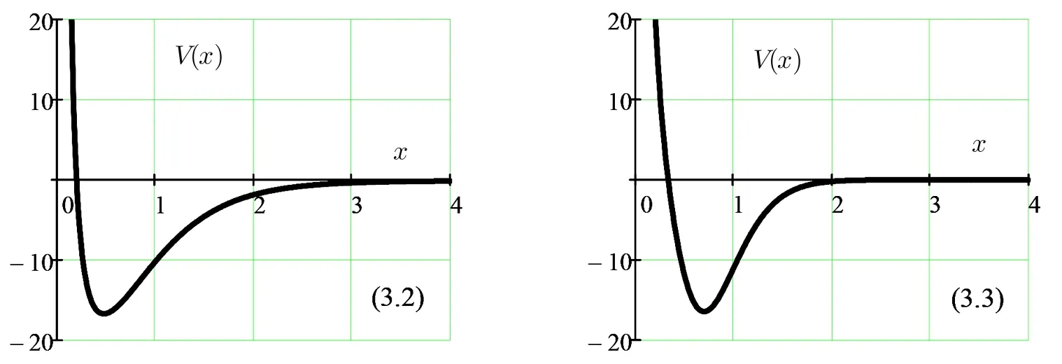
Fig.9 Plot of the potential function V(x)of Subsec.5.2.2 for the physical parameters{V2,γ,µ,a}={λ2,−7,2,2}.The second and third methods produce stable results for any value of the basis size N.However,these two results are not identical.The first and fourth methods produce results(not shown)that vary with the size of the basis and none agrees with the other two methods.The designation(3.n)means that the sub- figure was obtained using the n-th method introduced in section(3.n).

We end this subsection with a comment on the accuracy of the numerical results obtained by the four methods as shown in Figs.8 and 9.Recently,we considered the solution of the wave equation in the“Tridiagonal Representation Approach”[13]where we encountered a potential function with the following properties:

•One of its terms isV2/sinh2(λx).

•The expansion coefficients of the corresponding wavefunction in the basis(50)satisfy a three-term recursion relation with recursion coefficients that are almost identical to the matrix elements of the kinetic energy operator in Eq.(51).

That potential isV(x) =V2/sinh2(λx)+V1/cosh2(λx)+V0,which is the hyperbolic Poschl–Teller potential.We found a perfect match between the result of the second method and this potential for a proper choice of potential parametersV1andV0.

6 Conclusion

One of the advantages of reformulating quantum mechanics without a potential function is to enlarge the class of analytically describable systems(i.e.,exactly solvable problems).In this reformulation,orthogonal polynomials in the energy variable play the role of the potential function in standard quantum mechanics.They contain all the physical information about the system both structural and dynamical.Thus,the properties of these polynomials(e.g.,weight function,asymptotics,recursion relation,distribution of zeros,orthogonality,etc.)determine the features of the physical system.To establish a correspondence between the new formulation and the conventional one,we tried to reconstruct the potential function using only elements of the new formulation like the recursion relation of the energy polynomials and theL2basis used.There is no a priori guarantee that such reconstruction could be achieved unless a stringent requirement is placed on the basis and the sought after potential function whereby the matrix representation of the wave operator in the chosen basis is tridiagonal and symmetric.If so,then we will be able to recover the potential function either exactly by analytic means or approximately by numerical schemes.In this work,we did establish such procedure that was proven viable.

Acknowledgements

The support by the Saudi Center for Theoretical Physics(SCTP)during the progress of this work is highly appreciated.

Appendix A:Gauss Quadrature

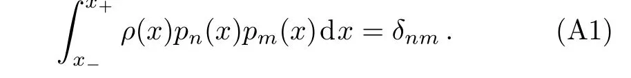
Let{pn(x)}∞n=0be a complete set of orthonormal polynomials over some interval in con fi guration spacex∈[x−,x+]withρ(x)being the normalized weight function.That is, ∫

They satisfy the following symmetric three-term recursion relation

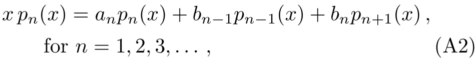
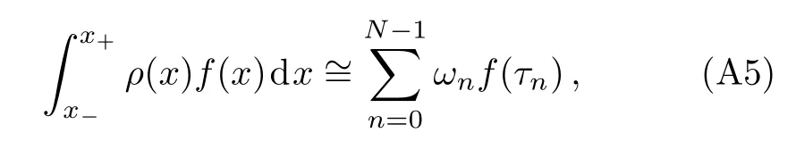
withbn/=0,p0(x)=1 andp1(x)=αx+β.Ifα=b−10andβ=−a0b−10,then we call these the “polynomials of the fi rst kind”.Let us construct theN×Ntridiagonal symmetric matrix if rst kindpN(x).Now,Gauss quadrature integral approx-

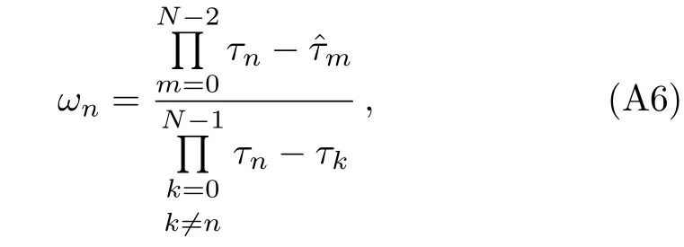
Let the polynomial variablexbe related to the con fi guration space coordinaterbyx=x(λr),whereλis a length scale parameter.Now,many of the basis elements in this con fi guration space are written in terms of orthonormal the integral(15)in Subsec.3.1 could be evaluated as follows

whereUn=(VΛWΛT)n0.

Appendix B:Relevant Energy Polynomials

For ease of reference,we de fi ne in this Appendix the three orthogonal energy polynomials that are relevant to our current study and give their main properties.We choose the orthonormal version of these polynomials and give their discrete versions that are used as expansion coeきcients of the bound states.

B1 The two-parameter Meixner–Pollaczek polynomial

The orthonormal version of this polynomial is written as follows(see pages 37–38 of Ref.[14])

whereyis the whole real line,µ＞0 and 0＜θ＜π.This is a polynomial inywhich is orthonormal with respect to the measureρµ(y,θ)dy.That is,

These polynomials satisfy the following symmetric threeterm recursion relation

The generating function associated with these polynomials is written as

The asymptotics(n→∞)is(see,for example,the Appendix in Ref.[2])

which is in the required general form given by Eq.(3)because then-dependent termyln(2nsinθ)in the argument of the cosine could be ignored relative tonθsince lnn≈o(n)asn→∞.The scattering amplitude in the asymptotics(B6)shows that a discrete in finite spectrum occur ifµ+iy=−m,wherem=0,1,2,...Thus,the spectrum formula associated with this polynomial isy2=−(m+µ)2and bound states will be written as in Eq.(4)where the discrete version of this polynomial is the Meixner polynomial whose normalized version is written as(see pages 45–46 in Ref.[14])

where 0＜β＜1.It satis fies the following recursion relation

B2 The three-parameter continuous dual Hahn polynomial

The normalized version of this polynomial is(see pages 29–31 of Ref.[14])

The asymptotics(n→∞)is(see,for example,the Appendix in Ref.[2])

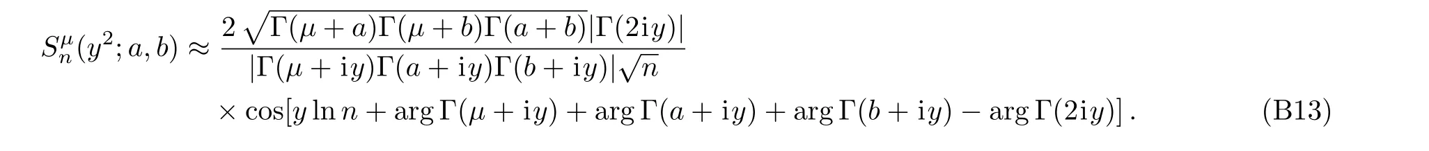
Noting that lnn≈o(nξ)for anyξ＞0,then this result is also in the required general form given by Eq.(3).The scattering amplitude in this asymptotics shows that a discrete finite spectrum occur ifµ+iy=−m,wherem=0,1,2,...,NandNis the largest integer less than or equal to−µ.Thus,the spectrum formula associated with this polynomial isy2=−(m+µ)2and the discrete version of this polynomial is the dual Hahn polynomial whose normalized version is written as(see pages 34–36 in Ref.[14])

The associated normalized discrete weight function is

B3 The four-parameter Wilson polynomial

wherey＞0 and the parameters{µ,ν,a,b}are positive except for a pair of complex conjugates with positive real parts.This is a polynomial iny2whose orthonormal version is written as

It is orthonormal with respect to the measureρµ(y;a,b)dywhere the normalized weight function reads as follows

It also satis fies the following symmetric three-term recursion relation

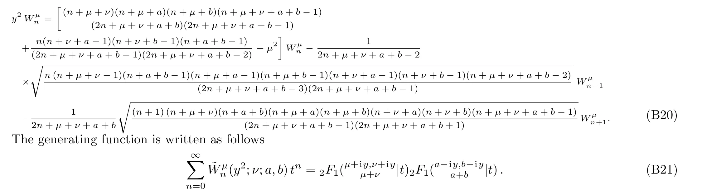
The asymptotics(n→∞)is(see,for example,Appendix B in Ref.[3])

and A(z)= Γ(2z)/Γ(µ+z)Γ(ν+z)Γ(a+z)Γ(b+z).Again,noting that lnn≈o(nξ)for anyξ＞0,then this result is also in the required general form given by Eq.(3).The scattering amplitude in this asymptotics shows that a discrete finite spectrum occur ifµ+iy=−m,wherem=0,1,2,...,NandNis the largest integer less than or equal to−µ.Thus,the spectrum formula associated with this polynomial isy2=−(m+µ)2and the discrete version of this polynomial is the Racah polynomial which we can write as(see pages 26–29 in Ref.[14])

wheren,m=0,1,2,...,Nand the parameter constraints areα＞−1,γ＞−1,β＞N−1.It satis fies the following recursion relation

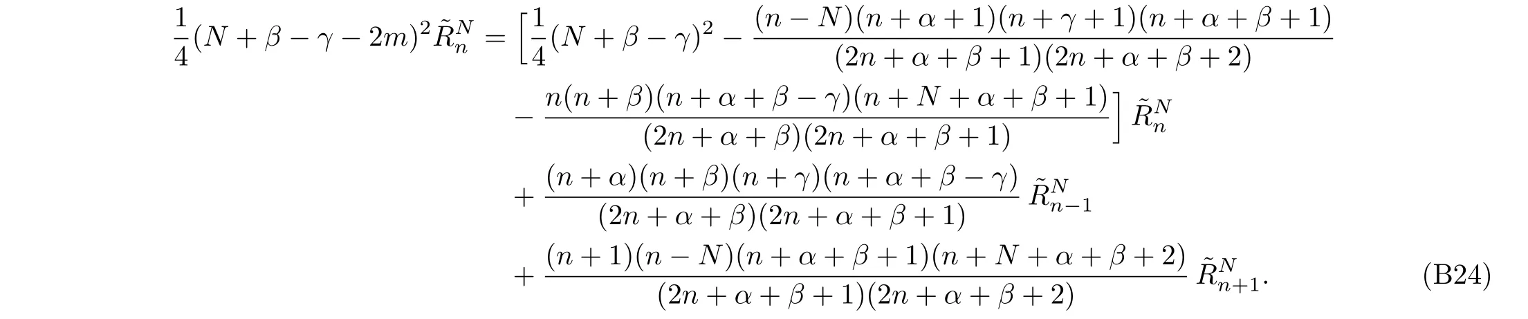
The discrete orthogonality relation reads as follows

and the orthonormal version of the discrete Racah polynomial is

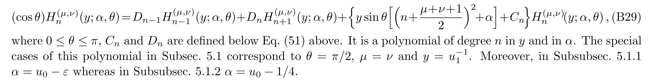
B4 New orthogonal polynomial

The orthogonal polynomial whose three-term recursion relation is given by either Eq.(44)or Eq.(49)is not found in the mathematics literature.Its properties(weight function,generating function,orthogonality,asymptotics,etc.)are yet to be derived analytically.Nonetheless,a generalized version of this polynomial,which is very relevant to various problems in physics,has already been encountered in the physics literature(see,for example,article Ref.[15]and references therein).This generalized polynomial is a four-parameter polynomial that was referred to as the“dipole polynomial” and is designated byH(µ,ν)n(y;α,θ).It satis fies the following symmetric three-term recursion relation

[1]A.D.Alhaidari,Quantum Physics Letters 4(2015)51.

[2]A.D.Alhaidari and M.E.H.Ismail,J.Math.Phys.56(2015)072107.

[3]A.D.Alhaidari and T.J.Taiwo,J.Math.Phys.58(2017)022101.

[4]See,for example,R.De,R.Dutt,and U.Sukhatme,J.Phys.A 25(1992)L843.

[5]J.F.Wang,X.L.Peng,L.H.Zhang,et al.,Chem.Phys.Lett.686(2017)131.

[6]C.S.Jia,C.W.Wang,L.H.Zhang,et al.,Chem.Phys.Lett.676(2017)150.

[7]X.Q.Song,C.W.Wang,and C.S.Jia,Chem.Phys.Lett.673(2017)50.

[8]C.S.Jia,L.H.Zhang,and C.W.Wang,Chem.Phys.Lett.667(2017)211.

[9]R.W.Haymaker and L.Schlessinger,The Pade Approximation in Theoretical Physics,ed.G.A.Baker and J.L.Gammel,Academic Press,New York(1970).

[10]P.C.Ojha,J.Phys.A 21(1988)875.

[11]A.D.Alhaidari and H.Bahlouli,J.Math.Phys.49(2008)082102.

[12]H.Bahlouli and A.D.Alhaidari,Physica Scripta 81(2010)025008.

[13]See subsection 3.2.1 in:A.D.Alhaidari,J.Math.Phys.58(2017)072104.

[14]R.Koekoek and R.Swarttouw,The Askey-Scheme of Hypergeometric Orthogonal Polynomials and Its q-Analogues,Reports of the Faculty of Technical Mathematics and Informatics,No.98–17,Delft University of Technology,Delft(1998).

[15]A.D.Alhaidari,Orthogonal Polynomials Derived from the Tridiagonal Representation Approach,arXiv:1703.-04039v2[math-ph],Submitted.