An Initial-Boundary Value Problem for Parabolic Monge-Amp`ere Equation in Mathematical Finance

Ming LI Changyu REN

1 Introduction

In[1],an optimal investment problem was proposed on the time interval[0,T].They used variables r,b,σ to describe the financial market.The attitude of the investors at the terminal time T for risk and interest can be describe by the utility function g(y).The goal is to search the optimal portfolio,and to achieve the maximum profit for investors.In[1],the following model was deduced to solve the above problem:

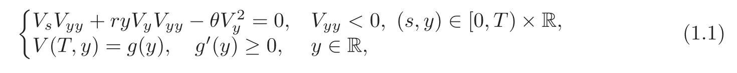
where V =V(s,y)is the undetermined function and r,b,σ are given constants,satisfying r≥ 0,σ ＞ 0,b−r＞ 0,Usually,we can assume that g(y)=1 − e−λy,where λ is some positive constant.In[2–3],the authors studied problem(1.1)and got the existence and uniqueness of smooth solution.

Note that the variable y in(1.1)means“the initial capital for investors”.Then,it is obvious that,for y ＜ 0,the investors can not invest anything.Meanwhile,“the initial capital” has to be finite.For the sake of using in the real world,we only consider the initial-boundary value problem in the domain[0,T)×(0,X).In this paper,we discuss the classical solution for the following problem:

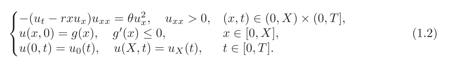
Here,we have used transformation(s,y)=(T−t,x),V(s,y)=−u(x,t)in(1.1).

By the way,from the viewpoint of partial differential equations,these problems are still valuable to discuss.In the famous work of Caffarelli-Nirenberg-Spruck[4]for Monge-Amp`ere equations,they proved the existence of the strictly convex solution to the following problem:

with the requirement of strictly convexity and the increasing condition:

As Krylov[5]pointed out that the corresponding parabolic problem matching(1.3)should be

Since we need to use the method of[4],we also require the condition appearing in(1.4)(also see[7]):

It is obvious that,for r=0,(1.2)becomes the type of(1.5),where n=1,detD2xu=uxx.But the requirement(1.6)can not be finished for the right-hand side of the problem(1.2)which may even be zero.

To overcome the difficulties,we observe that we can construct a sub-solution if the data of our problem satisfy appropriate conditions.Then,we derive the needed a prior estimates and use the degree theory to obtain the existence of the smooth solutions.

2 Preliminaries

For the equation(1.2)with a given function in the right-hand side,namely,the initialboundary value problem of the parabolic Monge-Amp`ere equation is

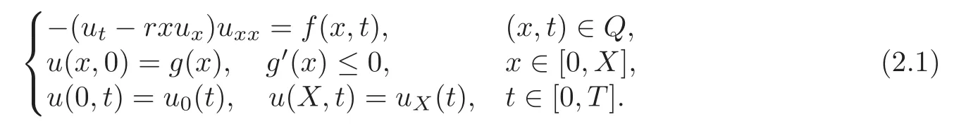
In this section we use Q to denote(0,X)×[0,T].

We assume that

(h1)There exist some constants α∈(0,1),μ＞0,such that

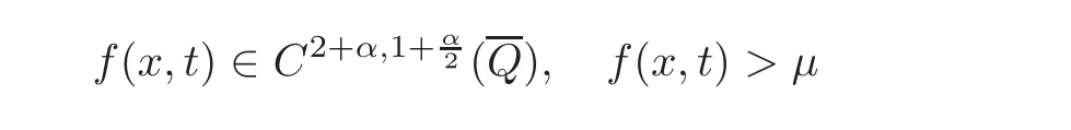
in Q.

(h2)g(x)∈ C4+α([0,X])satisfies g′′(x)≥ μ in[0,X],and u0(t),uX(t)∈ C2+α([0,T])satisfy

(h3)The data of problem(2.1)satisfy the compatibility conditions up to the second order.

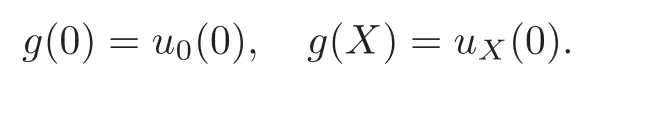
The compatibility condition is necessary for parabolic equations,which is one of the main differences to the elliptic type.The key point is that the initial data of the problem satisfy the smooth conditions at corner points.For instance,the 0th-order compatibility condition is

The 1st order compatibility condition is

Using the method in[6],by some modification,we can get the following result.

Theorem 2.1 If conditions(h1)–(h3)hold,then the problem(2.1)has a unique solution

3 Main Result

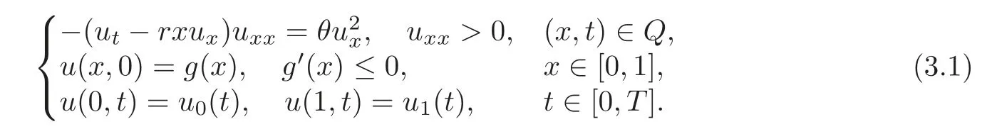
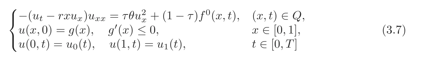
We note that(1.2)is invariant with the transformation x→Xx.Hence,without loss of generality,we can assume that X=1,and in the following,we use Q to denote(0,1)×(0,T].Then,(1.2)becomes

Now,we only consider the non-degenerate case of Equation(3.1).In our case,the solution should be called a strong convex monotonic function.Here,a function u(x,t)is called a strong convex monotonic function,if u(x,t)∈C2,1and

Since we will establish the existence of problem(3.1)inwe find the following necessary conditions:

(H1)There exist some constants α ∈ (0,1),μ ＞ 0,u0(t),u1(t)∈ C2+α([0,T]),and g(x)∈C4+α([0,1])satisfying −(t)≥ μ,−(t)−ru0(t)+ru1(t)≥ μ in[0,T],and g′(x)＜ 0,g′′(x)≥μ in[0,X].

(H2)The data of problem(3.1)satisfy compatibility conditions up to the second order.

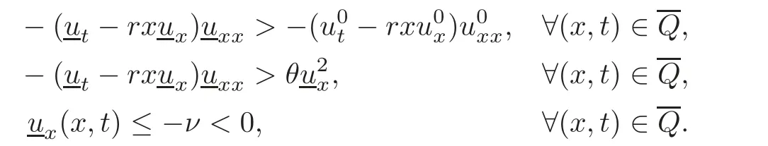
(H3)There exists some constant ν＞0 and two strong convex monotonic functions u0(x,t),satisfying

The following two lemmas give the sufficient conditions for(H3)to hold.

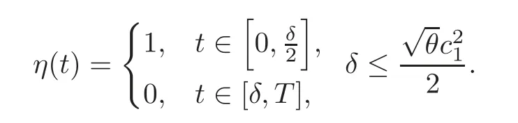
Lemma 3.1 If(H1)–(H2)and the following condition holds:

and for some constant c1＞0,we have

Then,we have some convex monotonic functionsatisfying

Proof We let

Hence,we get our result.

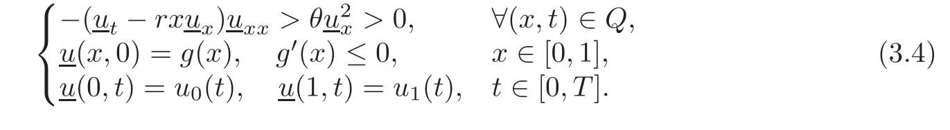
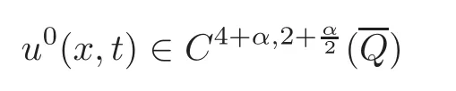
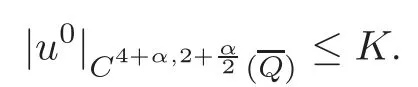
Lemma 3.2 If the condition in the above lemma is finished,then there is some strong convex monotonic function u0(x,t)∈ C4+α,2+α2(Q)satisfying

andHere the constant K only depends on the data of our problem(3.1).

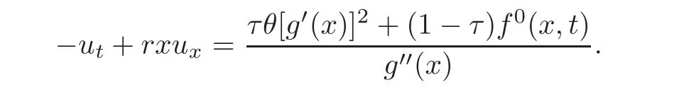
Proof Let

Then,it is obvious that A(x,t)

A(0,0)=A(1,0)=At(0,0)=At(1,0)=Ax(0,0)=Ax(1,0)=Axx(0,0)=Axx(1,0)=0.LetWe can check f0(x,t)＞0 inand

On the other hand,f0also satisfies the compatibility conditions up to the second order.

Using Theorem 2.1,we have a unique strong convex monotonic function

satisfying(3.5)and

Since u is the sub-solution for

By the proof of the above two lemmas,we have that the sufficient condition for(H3)is that Equation(3.1)has a strong convex monotinic sub-solution or that the following sub-solution

satisfies(x,t)≤ −c1,∀(x,t)∈In what follows,we use the degree theory to prove that the problem(3.1)has a strong convex monotonic solution.Let us consider the Banach space

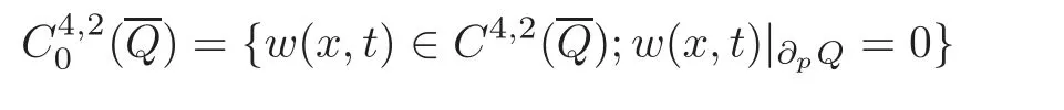
and its open subset,

S=is a strong cover solution}.

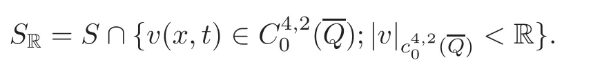
For a sufficiently large constant R,denote

We need the following lemma from[8].

Lemma 3.3 Denote Kρto be an interval in R1with radius ρ.Let w(x,t)in Q satisfy the Hlder condition for t with an exponential α and a Hlder constant μ1.Also assume that the derivative wxexists.It means that for any t ∈ [0,T],w(x,t)is Hlder continuous with respect to x.More explicitly,we have

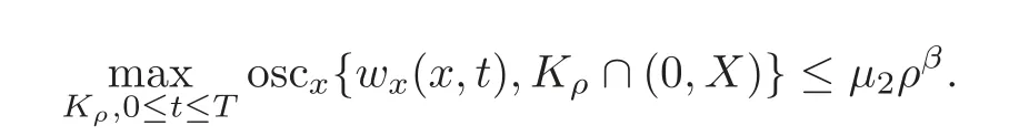
Then,the derivative wxin Q satisfies the Hlder condition for t with an exponential

The Hlder constant μ only depends on α,β,μ1,μ2.

Lemma 3.4 If(H1)–(H3)hold,then,for any v∈ S,τ∈ [0,1],the following problem

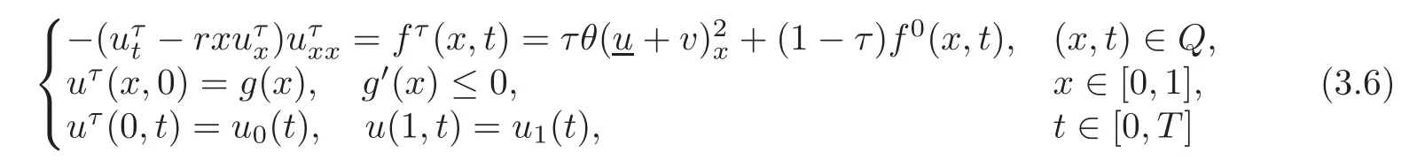
has a unique solutionwhere K0only depends on the data of the problem but not on τ.

Proof By Lemma 3.3,we know that the right-hand-side functionThen,it is easy to check that fτ(x,t)＞ 0 inand satisfies compatibility conditions up to the second order.Hence,by Theorem 2.1,we have the conclusion.

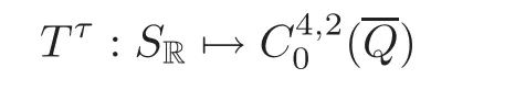
Lemma 3.5 Suppose that(H1)–(H3)hold.For any v ∈ S,the problem(3.6)has a unique solutionDenote vτ=uτ−Define some map Tτv=vτ.Then,we get that

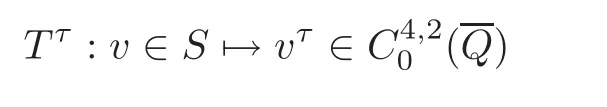
is a compact continuous map.

ProofBy Lemma 3.4 and the parabolic equation theory(see[10–11]),the image of thenot depending on τ,we have that Tτis a compact map.

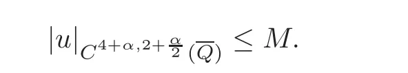
Lemma 3.6 There is a bounded constant M＞0,such that all solutions u(t,x)of the following problem

satisfy

Proof We note that uand

Hence,there is some bounded constant M1＞0,such that

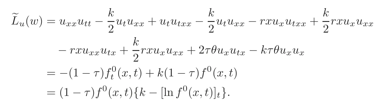
Let us estimate−ut.Define some linear operator

Consider the following test functionWe have

Ifwe haveBy the maximum principle,we have

Using the same linear operatorwe consider another two test functions

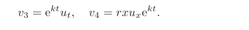
Direct calculation shows

If kwe getThen,we have

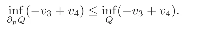
Hence,we obtain

Note that on{x=0}×[0,T],

On[0,x]×{t=0},we have

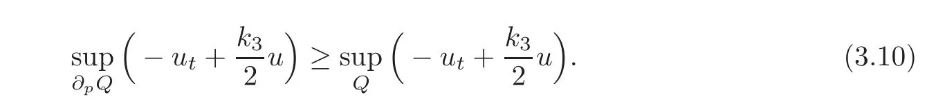
On{x=1}×[0,T],we have

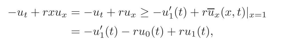
whereis the sup-solution of u defined by(3.8).Now combining(H1)–(H2),(3.9)–(3.11),there are some bounded constants c1,M2＞0,such that

Then,using Equation(3.7),there are bounded constants ν1＞ 0,M3＞ 0,such that

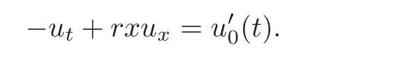
Taking the derivative with respect to t in(3.7),we have

The above equation is a linear equation about ut.Using Hlder estimates for bounded coefficient linear parabolic equations,we have

Combining(3.12)–(3.13)and using Equation(3.7),we have

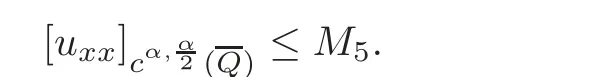
Combining all the results that we have obtained and using Schauder estimates,we have our conclusion.

Lemma 3.7 There exists some bounded constant R＞0,such that the operator I−Tτhas no zero on∂SR.

Proof By the definition of SR,we know that there exists no solution of Equation(3.7)on|v|C4,2=R.In what follows,we will have no solution of Equation(3.7)on∂SR,either.Suppose that u satisfies(3.7)on∂SR.Then,we have u≥and at least one of the following three cases holds:u=holds at some interior point of Q;(u−)x|x=0=0;(u−u)x|x=1=0.By the maximum principle and Hopf lemma(as Theorem 3 in[9]),we have τ＞0.But we also have

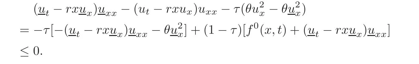
Since τ＞0,the equality will not appear in the above inequality.Again using the maximum principle and Hopf lemma,we have u≡u,which is a contradiction.Now,we can prove the main theorem.

Theorem 3.1 If conditions(H1)–(H3)hold,then the problem(3.1)only has a unique strong convex monotonic solution

Proof The maximum principle implies the uniqueness.We only need to discuss the existence.Since SRis a bounded subset in the Banach spacethe map

is a continuous compact operator.There is no zero for the operator I−Tτin∂SR.Thus,for τ∈[0,1],we can define the Leray-Schauder degree

By the homotopy invariant for the Leray-Schauder degree,we have

By the uniqueness,we have T0≡v0=u0−u,∀v∈SR.Hence,we have

which implies deg(I−T0,SR,0)=deg(I−v0,SR,0).Using the translation invariant and normalization of the Leray-Schauder degree,we have deg(I−v0,SR,0)=deg(I,SR,v0)=1.Thus,we obtain deg(I−T1,SR,0)=1.We have completed the proof.

AcknowledgementThe last author would like to thank his advisor Prof.Jixiang Fu for his help and encouragement.

[1]Yong,J.M.,Introduction to mathematical finance,in “Mathematical Finance –Theory and Applications”,Jiongmin Yong,Rama Cont,eds.,Beijing,High Education Press,2000,19–137.

[2]Wang,G.L.and Lian,S.Z.,An initial value problem for parabolic Monge-Amp`ere equation from investment theory,J.Partial Differential Equations,16(4),2003,381–383.

[3]Lian,S.Z.,Existence of solutions to initial value problem for a parabolic Monge-Amp`ere equation and application,Nonlinear Anal.,65(1),2006,59–78.

[4]Caffarelli,L.,Nirenberg,L.and Spruck,J.,The Dirichlet problem for nonlinear second-order elliptic equations I.Monge-Amp`ere equation,Communications on Pure and Applied Mathematics,37,1984,369–402.

[5]Krylov,N.V.,Boundedly inhomogenuous elliptic and parabolic equations,Izv.Akad.Nauk SSSR Ser.Mat.,46,1982,485–523;English transl.in Math.USSR Izv.,20,1983.

[6]Wang,G.L.,The first boundary value problem for parabolic Monge-Amp`ere equation,Northeast.Math.J.,3,1987,463–478.

[7]Wang,G.L.and Wang,W.,The first boundary value problem for general parabolic Monge-Amp`ere equation,J.Partial Differential Equations,3(2),1990,1–15.

[8]Ladyzhenskaja,O.A.,Solonnikov,V.A.and Ural’ceva,N.N.,Linear and quasilinear equations of parabolic type,American Mathematical Society,Providence,Ruode Island,1968.

[9]Murray,H.P.and Hans,F.W.,Maximum Principles in Differential Equations,Springer-Verlag,New York,Berlin,Heidelberg,Tokyo,1984.

[10]Lieberman,G.M.,Second Order Parabolic Differential Equations,World Scientific Publishing,Singapore,1996.

[11]Gilbarg,D.and Trudinger,N.S.,Elliptic Partial Differential Equations of Second Order,2nd edition,Grundlehren der Mathematischen Wissenschaften,Fundamental Principles of Mathematical Sciences,224,Springer-Verlag,Berlin,1983.