Simulation of Hot Shape Rolling of Steel in Continuous Rolling Mill by Local Radial Basis Function Collocation Method

U.Hanogluand B.Šarler,2,3

Simulation of Hot Shape Rolling of Steel in Continuous Rolling Mill by Local Radial Basis Function Collocation Method

U.Hanoglu1and B.Šarler1,2,3

The aim of this paper is to demonstrate the use of the novel Local Radial Basis Function Collocation Method(LRBFCM) [Šarler and Vertnik(2006)]in an industrial coupled thermo-mechanical problem of hot shape rolling of steel.The physical concept of such a large deformation problem is based on a two dimensional traveling slice model[Glowacki(2005)], which assumes deformation and heat flow only in the perpendicular direction to rolling.The solution is performed based on strong formulation.Elliptic Node Generation(ENG)is applied to reposition the nodes over a slice when necessary in order to sustain stability throughout the simulation.Coupled mechanical equilibrium steady Navier-Cauchy equations for a quasi-elastic material with temperature dependent material properties and the transient heat conduction equations are considered.The displacement and traction boundary conditions are assumed in the mechanical model and Dirichlet and Neumann boundary conditions in the thermal model,both specific for hot shape rolling.The solution procedure for mechanical model is based on local collocation on seven nodded influence domains with multiquadrics radial basis functions,augmented with the first order polynomials.Five nodded subdomains and explicit time-stepping are used in the thermal model.The elements of the thermomechanical LRBFCM model are tested on 3 different test cases:bending of a cantilever beam,compression and convective cooling.The results are compared with either FEM or analytical solution.The LRBFCM results of hot shape rolling of steel for a continuous 5 stand rolling mill are presented for the case of rolling of a rectangular billet from initial dimension 80 mm x 95 mm to a circular bar with a diameter of 60 mm.The advantage of the meshless method is in accuracy and straightforward node generation that does not require any polygonisation.The paper presents one of the increasingly emerging examples of the industrial use of LRBFCM.

Shape rolling,thermo-mechanics,meshless,radial basis functions,strong form,deformation,steel.

1 Introduction

Hot shape rolling of steel,that usually follows continuous casting of billets or blooms,provides different shapes of long products for various applications such as automotive industry,construction,shipbuilding, railway,etc.The demand is constantly changing due to the newly introduced designs and the production should be quickly adaptable.Respectively, computational modeling of the continuous casting as in[Lorbiecka,Vertnik, Gjerkeš,Manojlovic,Sencic,Cesar and Šarler(2009)]and/or hot rolling gains its importance for better understanding,control,and better insight into these processes.It helps to improve the quality,productivity,safety and environmental impact of the production.The principal goal of rolling simulation is to connect the process variables,such as the rolling speed,rolling temperature,rolling stand geometry,to the temperature,strain,strain rate,stress field in the billet,its microstructure with static and dynamic recrystallization,and calculation of the rolling torque and power.The modeling of rolling started with Hitchcock[Hitchcock(1935)]where he solved the problem of the roll deformation.A reasonably current state of the rolling technology and modeling can be perceived from[Lenard(2007);Lenard,Pietrzyk and Cser(1999)].

The majority of the simulations in solid mechanics are done by using Finite Element Method(FEM).This method requires meshing and re-meshing which might be problematic and time consuming,especially in case of rolling,where the shape is constantly and drastically changing.The advantages of using a meshless method over FEM are:it does not depend on node positioning as much as FEM,but FEM dramatically depends on mesh quality,a FEM model is usually overly stiff,which might give less accurate stress results.Meshless method is easier to code,it provides more flexibility in engineering applications,it is more capable of calculating large deformations, it is simple to pre-process, it allows to simply relocate the nodes and it has a high precision.

In the last decade,meshless numerical methods[Atluri(2004)]started to represent an appealing alternative to the classical numerical methods,such as FEM.Meshless method is a numerical technique that uses a set of arbitrary distributed nodes,both on the boundary and within the computation domain,to represent the solution of physical phenomena.The main feature of meshless methods is omission of the polygonalisation between the nodes which can be remarkably demanding,particularly in realistic 3D geometrical situations.The basis for meshless method discretization forms the meshless local Petrov-Galerkin method(MLPG)[Atluri and Shen(2005)].A review of applications of this method can be found in recen-t comprehensive review article[Sladek,Stanak,Han,Sladek and Atluri(2013)].Meshless methods are applied to large deformation problems such as forging and extrusion by[Hu,Yao and Hua(2007)]based on weak formulation.A strong form meshless solution procedure for plastic deformation problems is applied by[Guo,Nakanishi and Yokouchi(2005)].A comparison between weak and strong formulation is also made by[Batra and Zhang(2007)]for elastic deformation problems.In some publications,the use of strong form with Radial Basis Functions(RBF)is shown as a successful method[Kee,Liu,Zhang and Lu,(2008)]as well as using RBF with polynomial functions[Liu,Kee,Zhong,Li and Han,(2007)]in elastic cases.One of the simplest meshless methods,able to solve the fluid flow problems and solid mechanics problems is Local Radial Basis Function Collocation Method(LRBFCM),which is a special variant of MLPG.This method was first developed in[Šarler and Vertnik(2006)]for diffusion problems and in[Tolstykh and Shirobokov(2003)]for elasticity problems.The idea behind this method is to approximate the function and its derivatives locally over a set of neighboring nodes using RBFs[Buhmann(2004)]and to use collocation for determining the expansion coefficients.The method has been recently applied to numerous scientific and engineering problems,connected with fluid mechanics[Vertnik and Šarler(2009);Kosec,Založnik,Šarler and Combeau(2011)],simulation of continuous casting[Vertnik and Šarler(2014)]as well as solid mechanics[Hanoglu,Islam and Šarler(2011)].Thermoelasticity was by the LRBFCM recently coped in[Mavric and Šarler(2015)].In this paper,a basic model for simulation of hot shape rolling is performed by using LRBFCM.

2 Physical model

During the hot shape rolling,a billet goes through vertical and/or horizontal rolling stands to get the desired final shape.A major difference from the flat rolling originates from the fact that the roll surface has specific geometry such as oval or round.Hence,the simulation of hot shape rolling is a complex 3D problem.The problem can be reduced to 2D by taking into account the following assumptions:homogeneous compression(no deformation in rolling direction)and no heat flow in rolling direction.The problem is described in Cartesian coordinates with base vectorsix,iyandizwith coordinates px,py,pz.The calculations can be respectively done on 2D cross-sections which are parallel and aligned with the rolling direction,and perpendicular with base vectoriz.This solution concept is referred as the travelling slice method.The slice model is in the direction of rolling of the Lagrangean type,and perpendicular to rolling of the Eulerian type.This assumption is reasonable accurate when the heat flow in rolling direction can be neglected and the homogenous compression is assumed(planes remain planes).

Figure 1:Scheme of slice model of hot shape rolling.

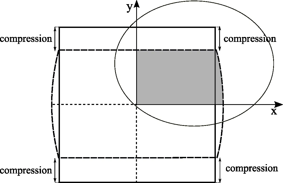
Figure 2:Symmetry of a rolled slice.Only the top right quarter is considered in the calculations.

2.1 Slice model assumptions

A scheme of a symmetrical quarter of the hot rolled billet is shown in Fig.1 with sketch of traveling slices.The temperature and the deformation field of a slice can be computed from the known position and time dependent boundary conditions.The homogenous compression assumption is based on planes remain planes criteria,therefore no deformation occur in rolling direction.There are two possible ways to analyze the simulation in terms of slices.A time incremental or position incremental method can be selected.In this research,predefined position increments∆z are used between the slices.The slice time is on the other hand associated with the position in the rolling direction pz.The pzcoordinate can be considered parabolic,while the pxand pycoordinates are elliptic.The slices form at the longitudinal coordinate of rolling pz=p0,at time t=t0and travel in the direction of theizwith the rolling speedv(t)and slice area A(t)(see Fig.1).For calculating the cooling intensity of the slice as a function of time,a connection between the pzcoordinate of the rolling mill and the corresponding time t is needed

2.2 Thermal model

The main aim of the thermal model is to calculate the thermal field over a slice by considering deformation which generates internal heat.The governing equation of the thermal model on a 2D slice is

with ρ,cp,T,t,k,˙Q standing for density,specific heat,temperature,time,thermal conductivity and internal heat generation rate per unit volume due to deformation,respectively.The boundary temperatures of the travelling slice were obtained from the Robin type boundary conditions over ΓRor Neumann type over ΓNin pointp,in 2D Cartesian coordinate systemp=pxix+pyiy,over the boundary Γ =ΓR∪ΓN.

at slice boundaries Γ,with h standing for the heat transfer coefficient to the air hairor to the roll hroll,standing for the ambient temperatureor the roll temperature.On the two symmetry axis q is set to 0,as shown in Fig.2.The heat source due to deformation is calculated as

2.3 Mechanical model

The main aim of the mechanical model is to calculate the displacement field of the slice due to deformation by the roll,in order to get the new shape of the slice.The governing equation of the mechanical model on a 2D slice is

where L is the derivative operator matrix with componentsis the vector of stresses,and b=[bxby]Tis the body force vector,considered b=0.Two dimensional plane strain model is assumed.The material is in the present basic rolling model assumed to be elastic,obeying plane strain assumption

where C is the stiffness matrix defined as

where E(T)and ν (T)are the temperature depended Young’s modulus and Poisson’s ratio respectively.The strain vector ε =[εxxεyyεxy]Tcan be written in terms of displacement vector as

Therefore,the strong formulation of deformation problem gives two individual balance equations in each principle direction on a 2D slice in terms of displacementu=[ux,uy]Twhich are

The boundary is divided into natural Γuand essential Γτpart Γ = Γu∪Γτ.The essential boundary conditions are considered between the slice and the roll and natural boundary condition are assumed at the boundary parts with no contact,as well as along the symmetry lines.The natural boundary conditions are defined in terms of displacement as

where in niis component of unit normal andis the prescribed shear stress component equal to 0 in case of no contact.The essential boundary condition is described as

Where uiis the displacement andis the prescribed displacement due to sticking boundary conditions with the roll.Corresponding boundary conditions for thermal and mechanical models,over a slice in contact with the roll,are shown in Fig.3.In order to be able to use the elastic model in rolling,an assumption is additionally made,which considers no elastic recovery(quasi-elastic material)after exit of each rolling stand.

3 Solution procedure

The coupled thermo-mechanical simulation is structured in the following way.First,collocation nodes are generated on the un-deformed slice with known initial temperature field and velocity.Boundary conditions are defined for the next slice regarding the roll contact and then,mechanical model is run for the displacement,strain and stress values.Afterwards,the thermal model is run for the same slice and a new temperature field is obtained.This process is repeated till the end of the rolling stand.Details of the solution process can be seen in Fig.4.

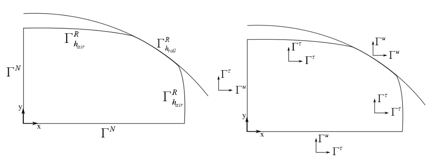
Figure 3:Scheme of boundary conditions.Left for the thermal model,right for the mechanical model when there is a contact with a roll.

3.1 Local radial basis function collocation method

LRBFCM is a very straightforward approach to solve partial differential equations.In order to get the results for a field ϕ,it needs to be approximated with interpolation function ψn(p)and coefficients αn

where the interpolation function is defined by scaled multiquadrics radial basis functions inside seven nodded influence domains(Nω=7),and first order polynomials(NP=3).

where xmax,ymax,xmea,ymearepresent maximum distance between the seven nodes inixandiydirections,and mean position of the seven nodes inixandiydirections,respectively.c is set to 32.The calculation of the coefficients αnis elaborated in[Šarler(2005)].The derivatives of the functions,needed in the solution,are calculated from the derivatives of the radial basis functions.

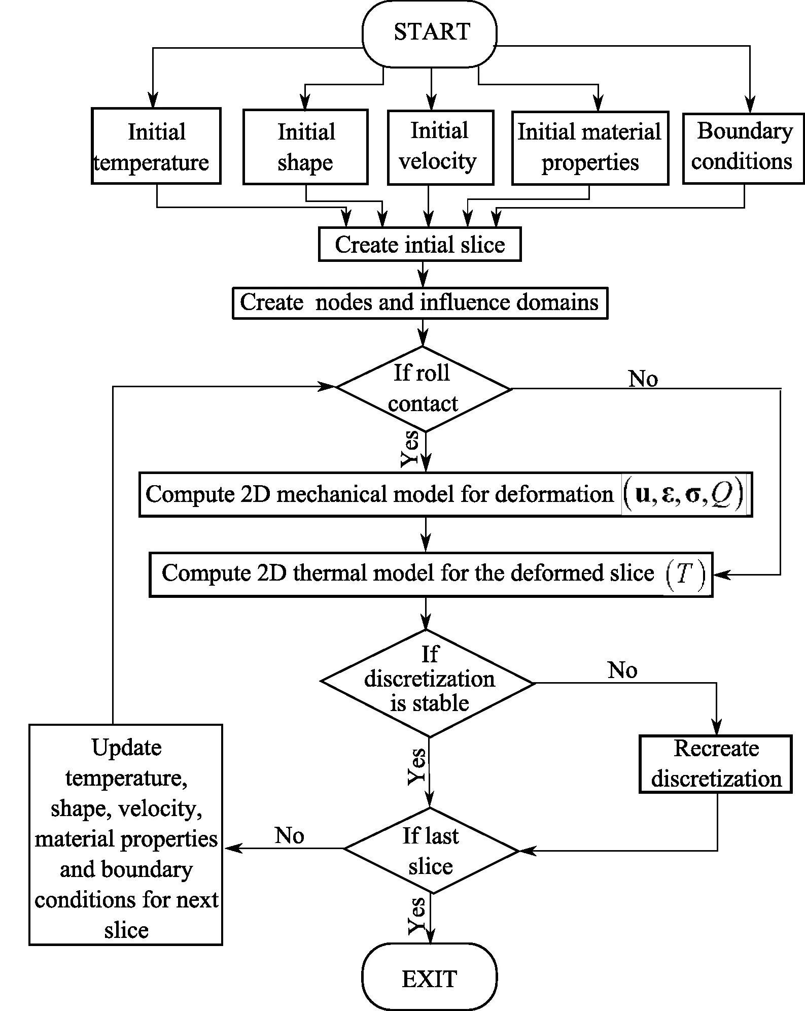
Figure 4:Flowchart of the thermo-mechanical simulation.

3.2 Solution of the thermal model

The discretization of the thermal model is performed in terms of temperature T as shown below.

where k(l,m)is a function returning the global node index taking influence domain index l and node index in an influence domain m.The thermal field is calculated whether there is a contact with the roll or not.We employ fully explicit(backward Euler)time discretization of temperature.

The discretized governing equation of the thermal model becomes

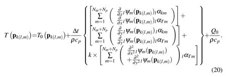
Neumann and Robin boundary conditions are also discretized in terms of temperature.

The solution of the thermal model requires inversion of a local interpolation matrix Ψ of the size Nω+NPfor each of the influence domain l which contains interpolation functions ψn(p),therefore,no global matrix is formed.

3.3 Solution of the mechanical model

The mechanical model is solved by expressing the displacements by radial basis functions

Therefore the governing equation is discretized as

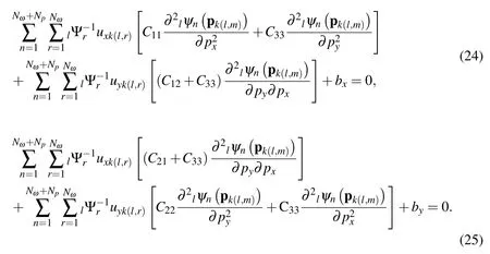
Traction boundary conditions are also discretized in terms of displacement as

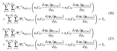
A set of global system of equations,composed from Eq.23,Eq.24,Eq.25 and Eq.26,can be written in a matrix formAU=BwhereAis a global solution(sparse)matrix,Uis a column vector of displacements andBis the adjacent vector.Hence,the displacements can be solved from these equations.The size of the solution matrix is 2 times the total number of collocation nodes.

3.4 Elliptic node generation

Large deformation problems such as hot shape rolling might create numerical instabilities during the solution procedure.The instabilities might be caused from severe collocation node displacements during the simulation.In order to overcome this issue,repositioning of the nodes can be done in between certain deformation steps.

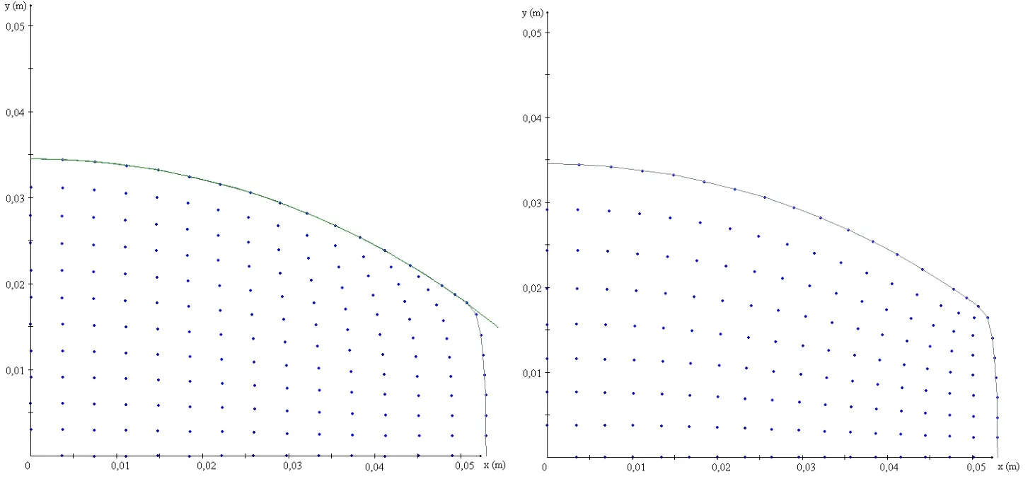
Figure 5:An example of regeneration of nodes with Elliptic Node Generation(ENG).Picture on the left is the deformation result after an oval rolling when uniform node distribution applied to a rectangle initially and picture on right is the same deformed slice when nodes are redistributed with ENG.

The nodes are newly generated on the new,deformed shape of the slice,based on elliptic node generation[Thompson,Soni,Weatherill(1999)].The previously calculated values are interpolated to the new position of the nodes by the simple Shepards’s interpolation method[Shepard(1968)].The calculated values of the old slice serve as initial values for the next slice.A demonstration of ENG is shown in Fig.4.In the calculations,Gauss-Seidel iteration is used and can be written for a global node ϑ(r,s)with latitudinal node order r and longitudinal node order s starting from the origin of the coordinate system.

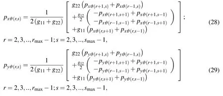
where the parameters g11,g12and g22are defined as

Shepard’s interpolation can be written for a field f(p)

where D is the Euclidean distance and λ is in the present work chosen as 2.

3.5 Groove geometry

A groove is a particular 3D shape which can have oval,diamond,box,round and many other types of shapes.A cross section of the groove has been calculated for each position of the slice towards the rolling direction.Thus,all the geometrical parameters are known for each groove such as seen on Figure 6.

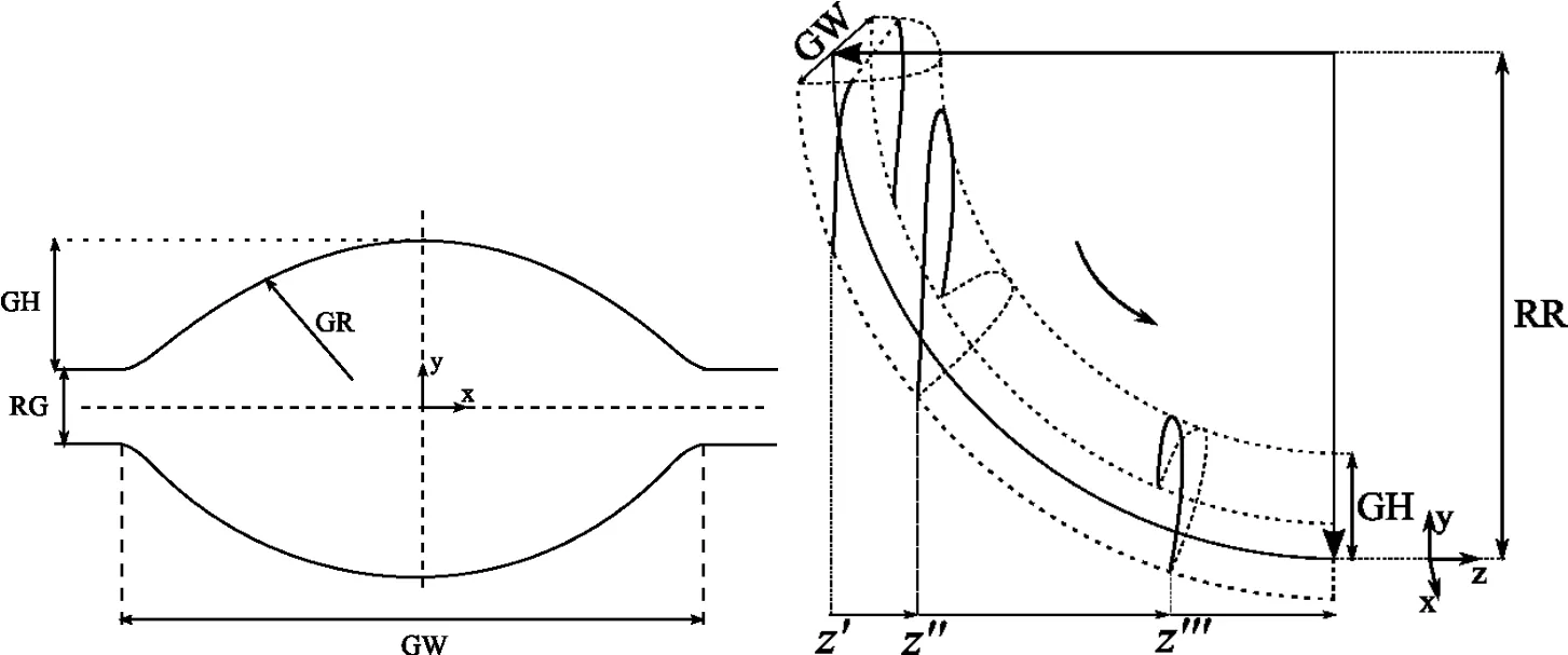
Figure 6:Horizontal oval groove dimensions.GH is the groove height,GR is the groove radius,GW is the groove width,RG is the roll gap and RR is the roll radius.

4 Numerical results

The LRBFCM is first tested for bending of a cantilever beam and compared with the analytical solution.Afterwards,a prescribed pressure is applied on a square material for compression.Thermal part of the numerical implementations is tested on convective cooling example.The last two examples are compared with FEM,calculated by DEFORM[DEFORM(2009)]code.Later,a complete rolling simulation is done based on a rolling schedule given in Tab.2 with given parameters in Tab.1.

4.1 Bending of a cantilever beam

A deformation example,widely used for verification,is bending of a cantilever beam.Length of the beam L is 48 m and height H is 12 m.The traction applied at the end P=30Pa,Young’s modulus of the beam E=1000Pa and Poisson’s ratio ν=0.3.Boundary conditions on each side are explained below and shown in Fig.6.

The boundary conditions on the left side are taken from the analytical solution[Liu(2003)].

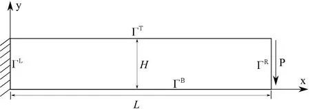
Figure 7:Scheme of bending of a cantilever beam problem.

The results calculated by LRBFCM are shown in Fig.8 and compared with analytical solution as in[Liu(2003)].Root mean square error(RMSE)of displacement values are calculated against the increasing number of the collocation nodes in Fig.9.

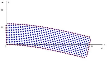
Figure 8:572 collocation nodes used in calculations(round points)by LRBFCM compared with analytical solution(squares)at the boundary points.

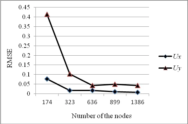
Figure 9:RMSE of displacements versus the number of the collocation nodes.

The shear stress at the end of the beam(x=L),can be obtained from the calculated displacements with LRBFCM and compared with analytical solution as in Figure 10.

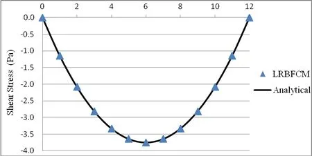
Figure 10:Shear stress at the end of the cantilever beam when x=L compared with the analytical solution.

4.2 Compression test compared with FEM

A 2 m × 2 m shaped material with Young’s modulus E=1 Pa and Poisson ratio ν=0.3 is chosen for the present example.Centre of the coordinate system is in the middle of the bottom line of the object.At the top,the prescribed pressure is applied towards the y direction,however the displacement in x direction is always fixed to 0.A definition of the problem is given in Fig.11.The results in this paper are compared with FEM[DEFORM(2009)]code.

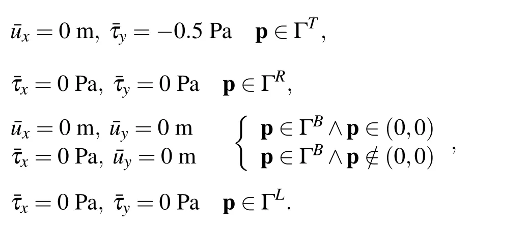
The deformation results calculated by LRBFCM and FEM are shown in Fig.12 and Fig.13 in terms of displacement vectors and displacement fields.

A further comparison of calculated strain components are made in Fig.14,Fig.15 and Fig.16 below and a very good agreement has been achieved.

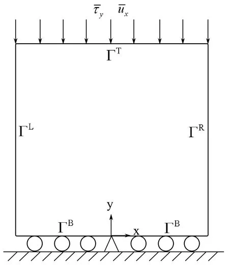
Figure 11:Scheme of the geometry and boundary conditions for compression tension examples.

Figure 12:Displacement vectors calculated by LRBFCM(on top)with 441 collocation nodes and FEM(at the bottom)with 196 quadrilateral finite elements.

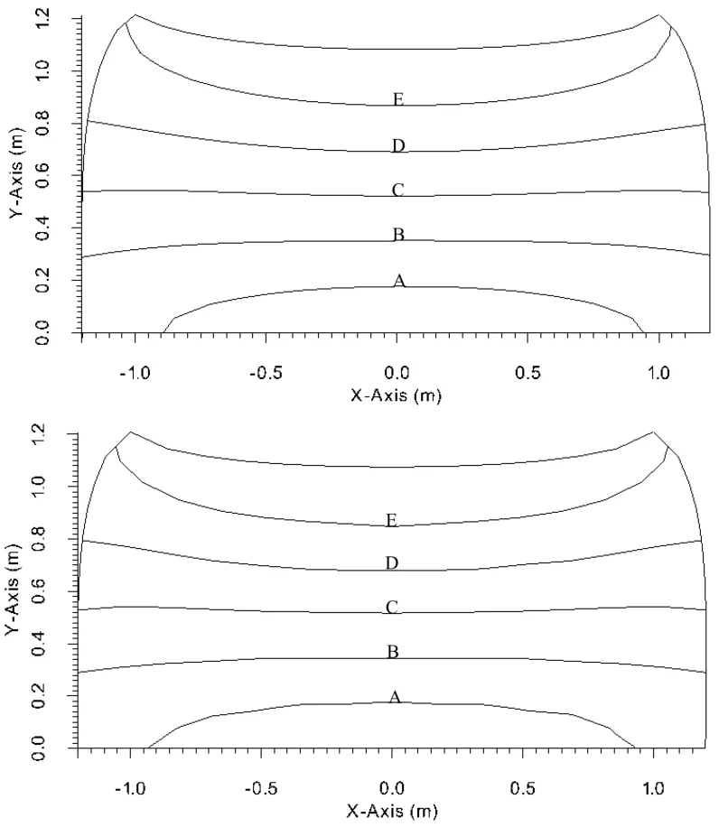
Figure 13:Comparison of displacement fields with LRBFCM(on top)and FEM(at the bottom).Lines represent A=0.154 m,B=0.308 m,C=0.462 m,D=0.617 m and E=0.771 m.

Figure 14:Comparison of εxxfields with LRBFCM(on top)and FEM(at the bottom).Lines represent A=0.0648,B=0.102,C=0.139 and D=0.176.

Figure 15:Comparison of εyyfields with LRBFCM(on top)and FEM(at the bottom).Lines represent A=-0.459,B=-0.436,C=-0.412 and D=-0.388.

Figure 16:Comparison of εxyfields with LRBFCM(on top)and FEM(at the bottom).Lines represent A=-0.152,B=-0.0914,C=-0.0305,D=0.0305,E=0.0914 and F=0.152.

4.3 Convective cooling compared with FEM

A square domain with 50 mm side is used for testing.The density is ρ=7450 kg/m3,specific heat is cp=630 J/kgK,thermal conductivity is k=29 W/mK.Uniformly distributed 676 discretization points are used across the domain.1076 elements are used in reference FEM.The time step in LRBFCM is set to 0.1 s and for FEM 1 s is used.The scheme of the problem is given in Figure 17.

Left and bottom boundaries are of the Neumann type where the prescribed heat flux is 0 W/m2.For the top and right boundaries Robin type of boundary condition is applied.

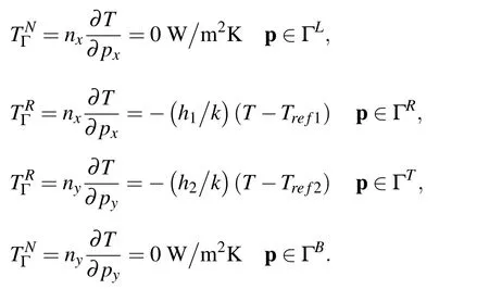
The initial temperature is set to 1000˚C,h1=20 W/m2K,h2=5000 W/m2K,Tref1=25˚C,Tref2=500˚C and˙Q=0 W/m3.The heat transfer coefficient on the top side is chosen in such a way to be consistent with the contact with the roll and the heat transfer coefficient of the right side imitates the heat flow to the air.

The simulation result at 10 s and 60 s are compared with FEM in Fig.18 and Fig.19 respectively.

As expected,excellent agreement has been achieved between LRBFCM and FEM for the thermal model.

4.4 Solution of hot shape rolling by LRBFCM

A complete rolling schedule is put on test and solution is obtained by LRBFCM.The process parameters are given in Tab.1.The slice positions towards the rolling direction have predefined distances in between such as 5 or 10 mm.The successive groove lines for each slice positions under each groove are drawn as well as the displacement vectors in figures Fig.20,Fig.21,Fig.22,Fig.23 and Fig.24.Initial cross section of the bloom is 80 mm×95 mm but due to symmetry,only the top right quarter is considered.The rolling simulation is carried out over 13 m long rolling schedule considering 1455 discrete slice positions.?

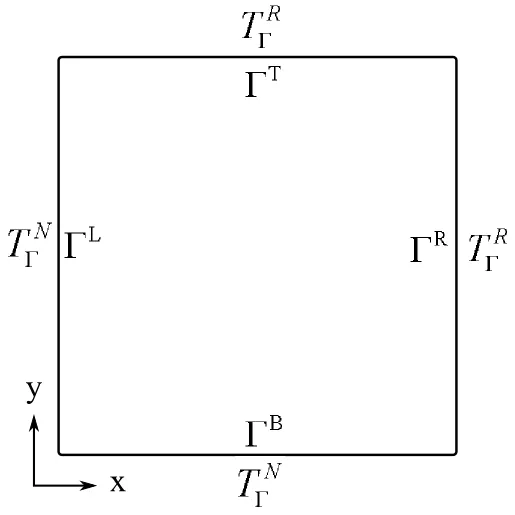
Figure 17:Scheme of the boundary conditions of the thermal test case.

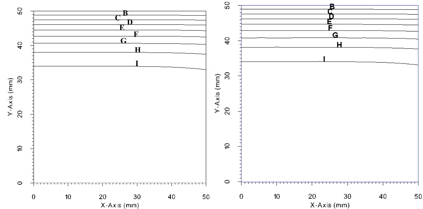
Figure 18:Thermal test case.Left:LRBFCM,Right:FEM at time 10 s.All of the sides have the length of 50 mm.Lines represent B=709 ˚C,C=745 ˚C,D=782 ˚C,E=818 ˚C,F=854 ˚C,G=891 ˚C,H=927 ˚C and I=964 ˚C.

Figure 19:Thermal test case.Left:LRBFCM,Right:FEM at time 60 s.All of the sides have the length of 50 mm.The contour lines represents B=620˚C,C=662˚C,D=703˚C,E=745˚C,F=787˚C,G=829˚C,H=871˚C and I=913˚C.

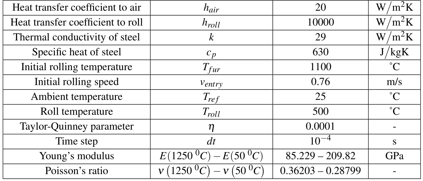
Table 1:Thermal and mechanical parameters used in calculations.

Table 2:Rolling schedule used in the simulation.

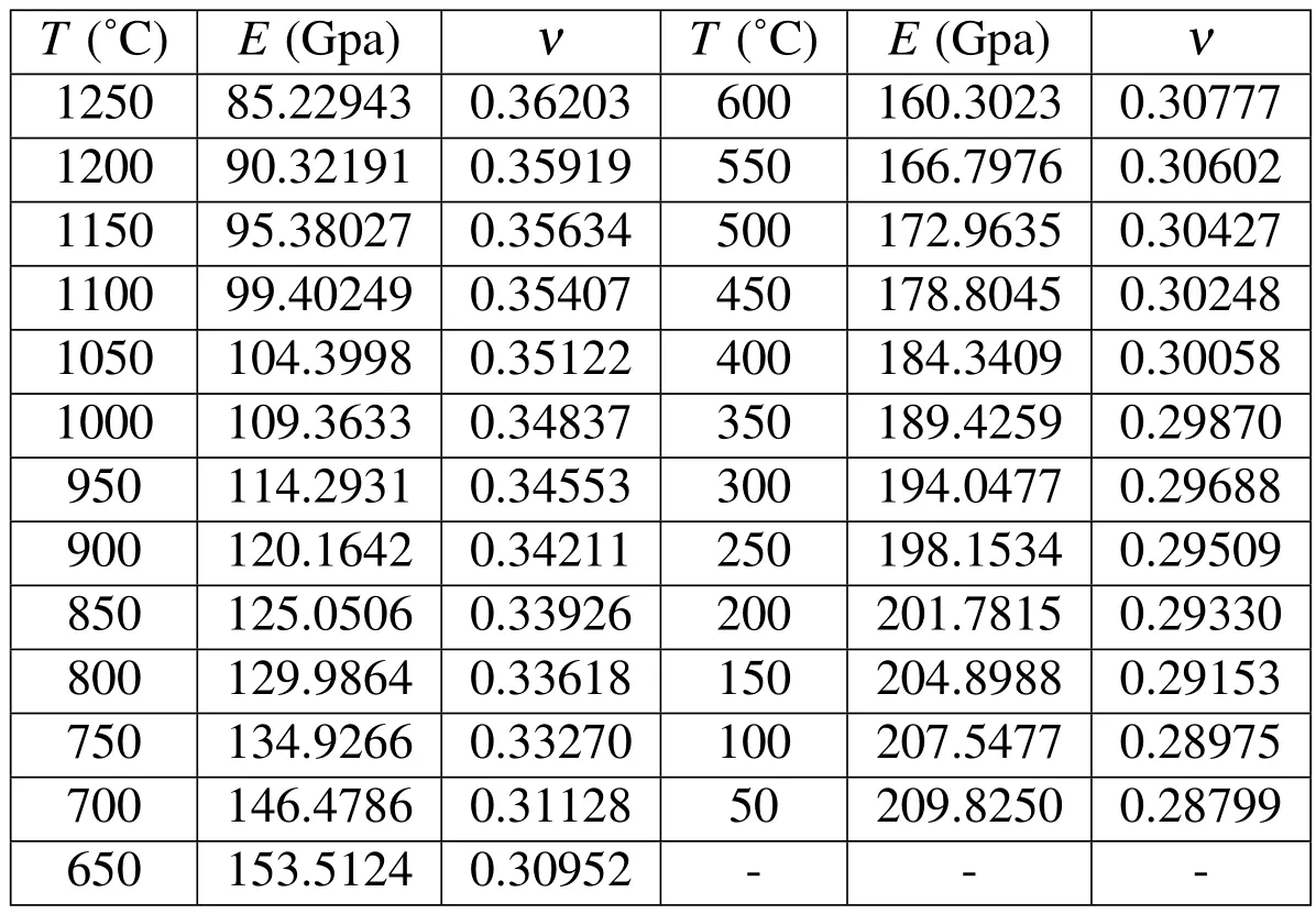
Table 3:Elastic material properties for 16MnCrS5 steel for corresponding temperature values used in hot shape rolling simulation.

The geometrical details of the rolling schedule are given in Tab.2.H and V stand for horizontal and vertical rolling stands in which the top and bottom rolls in a rolling stand are aligned horizontally or vertically.

The coupling of mechanical and thermal models is achieved through the temperature depended material properties,as given in Tab.3,which are used in the solution procedure of the mechanical model.

Figure 20:Displacement vectors at the exit of the first rolling stand.26 groove lines represent necessary deformation steps as a consequence of the process with 120 collocation nodes.

In the rolling simulation,except for the displacment vectors,initially 480 collocation nodes are uniformly distributed,after the exit from the first rolling stand ENG is applied and total number of collocation nodes becomes 340 and it is carried out with the same number untill the end of the simulation.The displacment fileds calculated by LRBFCM after exit of each rolling stand can be seen in Fig.25.

The temperature field calculated by LRBFCM at the exit of each rolling stand are shown in Fig 26,Fig.27 and Fig.28 below.As expected,heat loss is proportional to the roll contact area and duration.

Sensitivity studies of the thermal model during the rolling simulation based on increased roll temperature and increased heat transfer coefficient to the roll can be seen in Fig.29.The corresponding velocities of the slices towards the rolling direction at nominal conditions are shown in Fig.30 for each slice position.

Figure 21:Displacement vectors at the exit of the second rolling stand.16 groove lines represent necessary deformation steps as a consequence of the process with 112 collocation nodes.

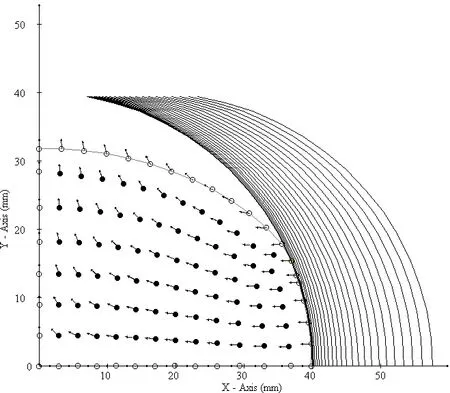
Figure 22:Displacement vectors at the exit of the third rolling stand.25 groove lines represent necessary deformation steps as a consequence of the process with 112 collocation nodes.

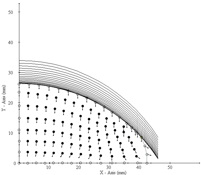
Figure 23:Displacement vectors at the exit of the fourth rolling stand.17 groove lines represent necessary deformation steps as a consequence of the process with 112 collocation nodes.

Figure 24:Displacement vectors at the exit of the fifth rolling stand.23 groove lines represent necessary deformation steps as a consequence of the process with 112 collocation nodes.

Figure 25:Contour graphs of displacement fields at the exit of each rolling stand starting from the initial shape(top-left)untill the 5throlling stand(bottom-right).The values are in mm.

Figure 26:Temperature field at the exit of the first rolling stand(on left)and the lines represent A=1060.04 ˚C,B=1068.03 ˚C,C=1076.02 ˚C,D=1084.02 ˚C,E=1092.01 ˚C and F=1100.00 ˚C.Temperature field at the exit of the second rolling stand(on right)are represented by values;A=1057.06 ˚C,B=1066.04 ˚C,C=1074.53 ˚C,D=1083.02 ˚C and E=1091.51 ˚C.

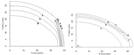
Figure 27:Temperature field at the exit of the third rolling stand(on left)and the lines represent A=1060.77 ˚C,B=1067.31 ˚C,C=1073.84 ˚C,D=1080.38 ˚C,E=1086.91 ˚C,F=1093.45 ˚C and G=1999.99 ˚C.Temperature field at the exit of the fourth rolling stand(on right)are represented by values;A=1058.24˚C,B=1066.58 ˚C,C=1074.91 ˚C,D=1083.25 ˚C,E=1091.58 ˚C and F=1099.92 ˚C.

Figure 28:Temperature field at the exit of the fifth rolling stand.The lines represent A=1048.63 ˚C,B=1055.02 ˚C,C=1061.40 ˚C,D=1067.78 ˚C,E=1074.17 ˚C,F=1080.56 ˚C and G=1086.94 ˚C and H=1093.32 ˚C.

Figure 29:Average slice temperatures in˚C versus the slice positions towards the rolling direction.Different thermal conditions are used and results are compared with nominal conditions.

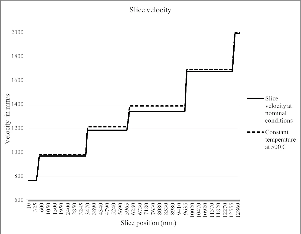
Figure 30:Velocity of slices versus the slice positions towards the rolling direction.The dashed line represents the results when slice temperature is kept constant at 500 ˚C.

5 Conclusions and future work

In this paper simulation of hot shape rolling is done by LRBFCM.This method is previously tested for bending of a cantilever beam problem with analytical solution,compression and convective cooling test results are compared with FEM.In the rolling simulation a coupled thermo-mechanical model is used for plane strain slice model results.The temperature depended material properties are obtained for 16MnCrS5 steel.The simulation is carried out over 13 m long rolling mill which includes 5 rolling stands.The results are calculated through 1455 slice positions and in this paper results after each rolling stand are given in terms of displacement and temperature fields.Two sensitivity studies are done to see the behavior of the solution procedure based on average slice temperature and slice velocities.It is shown that LRBFCM is a stable method to simulate a complete rolling schedule.Different material types such as ideal plastic will be included in the simulation in our future work.The non-linear behavior of the materiel models used in the ideal plastic deformation requires additional effort to achieve stable solutions.This complexity is expected to be solved by Newton-Raphson iteration method[Chen and Han(1988)].However,the solution time is also expected to increase since this process will be repeated in every deformation step through the simulation.New rolling schedules with different parameters will be incorporated in future industrial rolling analyses.

Acknowledgement:The authors wish to acknowledge Slovenian Grant Agency for the support in the framework of Young Researcher Program,program group P2-03679 and project L2-6775.

Atluri,S.N.(2004):The Meshless Local Petorov-Galerkin Method(MLPG),Tech.Science Press.

Atluri,S.N.;Shen,S.(2005):The basis of meshless domain discretization:the meshless local Petrov-Galerkin(MLPG)method.Advances in Computational Mathematics,vol.23,pp 73-93.

Batra,R.C.;Zhang,G.M.(2007).SSPH basis functions for meshless methods,and comparison of solutions with strong and weak formulations.Computational Mechanics,vol.41,pp.527-545.

Buhmann,M.D.(2004):Radial Basis Functions,Cambridge University Press.

DEFORM.(2009):Scientific Forming Technologies Corporation,Version 10.1,http://www.deform.com.

Chen,W.F.;Han,D.J.(1988):Plasticity for Structural Engineers,Springer-Verlag.

Glowacki,M.(2005):The mathematical modeling of thermo-mechanical processing of steel during multi-pass shape rolling.Journal of Materials Processing Technology,vol.168,pp.336-343.

Guo,Y.;Nakanishi,K.;Yokouchi,Y.(2005):A non-linear rigid-plastic analysis for metal forming problem using the rigid-plastic point collocation method.Advances in Engineering and Software,vol.36,pp.234-242

Hanoglu,U.;Islam,S.;Šarler,B.(2011):Thermo-mechanical analysis of hot shape rolling of steel by a meshless method.Procedia Engineering,vol.10,pp.3173-3178.

Hitchcock,J.H.(1935):Roll Neck Bearings.ASME Research publication.

Hu,W.;Yao,L.G.;Hua,Z.Z.(2006):Parallel point interpolation method for three-dimensional metal forming simulation.Engineering Analysis with Boundary Elements,vol.31,pp.326-342.

Kee,B.B.T.;Liu,G.R.;Zhang,G.Y.;Lu,C.(2008):A residual based error estimator using radial basis functions.Finite Elements in Analysis and Design,vol.44,pp.631-645.

Kosec,G.;Založnik,M.;Šarler,B.;Combeau,H.(2011):A meshless approach towards solution of macrosegregation phenomena.CMC:Computers Materials and Continua,vol.22,pp.169-196.

Lenard,J.G.(2007):Primer on flat rolling,Elsevier.

Lenard,J.G.;Pietrzyk,M.;Cser,L.(1999):Mathematical and Physical Simulation of the Properties of Hot Rolled Products,Elsevier.

Liu,G.R.(2003):Mesh Free Methods,CRC Press.

Liu,G.R.;Kee,B.B.T.;Zhong,Z.H.;Li,G.Y.;Han,X.(2007):Adaptive meshfree methods using local nodes and radial basis functions,Proceedings of Enhancement and Promotion of Computational Methods in Engineering and Science,Sanya,Hainana,China,August 21-23,pp.71-86.

Lorbiecka,A.Z;Vertnik,R.;Gjerkeš,H.;Manojlovic,G.;Sencic,B.;Cesar,J.;Šarler,B.(2009).Numerical modeling of grain structure in continuous casting of steel.CMC:Computers Materials and Continua,vol.8,pp.195-208.

Mavric,B.;Šarler,B.(2015):Local radial basis function collocation method for linear thermoelasticity in two dimensions.International Journal of Numerical Methods in Heat&Fluid Flow,vol.25,pp.1488-1510.

Šarler,B.(2005):A radial basis function collocation approach in computational fluid dynamics.CMES:Computer Modeling in Engineering and Sciences,vol.7,pp.195-193.

Šarler,B.;Vertnik,R.(2006):Meshfree local radial basis function collocation method for diffusion problems. Computers and Mathematics with Application,vol.51,pp.1269-1282.

Sladek,J.;Stanak,P.;Han,Z.D.;Sladek,V.;Atluri S.N.(2013).Applications of the MLPG Method in Engineering&Sciences:A Review.CMES:Computer Modeling in Engineering&Sciences,vol.92,pp.423-475.

Shepard,D.(1968):A two-dimensional interpolation function for irregularly spaced data.Proceedings of the 23rd Association for Computing Machinery(ACM)national conference,Las Vegas,USA,August 27-29.

Thompson,J.F.;Soni,B.K.;Weatherill,N.P.(1999):Handbook of Grid Generation,CRC Press.

Tolstykh,A.I.;Shirobokov,D.A.(2003):On using radial basis functions in a“finite difference mode”.Computational Mechanics,vol.33,pp.68-79.

Vertnik,R.;Šarler,B.(2009):Solution of incompressible turbulent flow by a mesh-free method.CMES:Computer Modeling in Engineering and Sciences,vol.44,pp.65-96.

Vertnik,R.;Šarler,B.(2014):Solution of continuous casting of steel benchmark test by a meshless method.Engineering Analysis with Boundary Elements,vol.45,pp.45-61.

1University of Nova Gorica,Nova Gorica,Slovenia.

2IMT,Ljubljana,Slovenia.

3Corresponding author:Professor Božidar Šarler.

E-mail:bozidar.sarler@imt.si;bozidar.sarler@ung.si