Double Optimal Regularization Algorithms for Solving Ill-Posed Linear Problems under Large Noise

Chein-Shan Liu,Satya N.Atluri

Double Optimal Regularization Algorithms for Solving Ill-Posed Linear Problems under Large Noise

Chein-Shan Liu1,Satya N.Atluri2

A double optimal solution of ann-dimensional system of linear equations Ax=b has been derived in an affinem-dimensional Krylov subspace withm≪n.We further develop adouble optimal iterative algorithm(DOIA),with the descent direction z being solved from the residual equation Az=r0by using its double optimal solution,to solve ill-posed linear problem under large noise.The DOIA is proven to be absolutely convergent step-by-step with the square residual error‖r‖2= ‖b−Ax‖2being reduced by a positive quantity ‖Azk‖2at each iteration step,which is found to be better than those algorithms based on the minimization of the square residual error in anm-dimensional Krylov subspace.In order to tackle the ill-posed linear problem under a large noise,we also propose a noveldouble optimal regularization algorithm(DORA)to solve it,which is an improvement of the Tikhonov regularization method.Some numerical tests reveal the high performance of DOIA and DORA against large noise.These methods are of use in the ill-posed problems of structural health-monitoring.

Ill-posed linear equations system,Double optimal solution,Affine Krylov subspace,Double optimal iterative algorithm,Double optimal regularization algorithm.

1 Introduction

A double optimal solution of a linear equations system has been derived in an affine Krylov subspace by Liu(2014a).The Krylov subspace methods are among the most widely used iterative algorithms for solving systems of linear equations[Dongarra and Sullivan(2000);Freund and Nachtigal(1991);Liu(2013a);Saad(1981);van Den Eshof and Sleijpen(2004)].The iterative algorithms that are applied to solve large scale linear systems are likely to be the preconditioned Krylov subspace methods[Simoncini and Szyld(2007)].Since the pioneering works of Hestenes(1952)and Lanczos(1952),the Krylov subspace methods have been further studied,like the minimum residual algorithm[Paige and Saunders(1975)],the generalized minimal residual method(GMRES)[Saad(1981);Saad and Schultz(1986)],the quasi-minimal residual method[Freund and Nachtigal(1991)],the biconjugate gradient method[Fletcher(1976)],the conjugate gradient squared method[Sonneveld(1989)],and the biconjugate gradient stabilized method[van der Vorst(1992)].There are a lot of discussions on the Krylov subspace methods in Simoncini and Szyld(2007),Saad and van der Vorst(2000),Saad(2003),and van der Vorst(2003).The iterative method GMRES and several implementations for the GMRES were assessed for solving ill-posed linear systems by Matinfar, Zareamoghaddam,Eslami and Saeidy(2012).On the other hand,the Arnoldi’s full orthogonalization method(FOM)is also an effective and useful algorithm to solve a system of linear equations[Saad(2003)].Based on two minimization techniques being realized in an affine Krylov subspace,Liu(2014a)has recently developed a new theory to find a double optimal solution of the following linear equations system:

where x∈Rnis an unknown vector,to be determined from a given non-singular coefficient matrix A ∈ Rn×n,and the input vector b ∈ Rn.For the existence of solution x we suppose that rank(A)=n.

Sometimes the above equation is obtained via ann-dimensional discretization of a bounded linear operator equation under a noisy input.We only look for a generalized solution x=A†b,where A†is a pseudo-inverse of A in the Penrose sense.When A is severely ill-posed and the data are disturbanced by random noise,the numerical solution of Eq.(1)might deviate from the exact one.If we only know the perturbed input data bδ∈Rnwith‖b−bδ‖≤δ,and if the problem is ill-posed,i.e.,the range(A)is not closed or equivalently A†is unbounded,we have to solve Eq.(1)by a regularization method[Daubechies and Defrise(2004)].

Given an initial guess x0,from Eq.(1)we have an initial residual:

Upon letting

Eq.(1)is equivalent to

which can be used to search the Newton descent direction z after giving an initial residual r0[Liu(2012a)].Therefore,Eq.(4)may be called theresidual equation.

Liu(2012b,2013b,2013c)has proposed the following merit function:

and minimized it to obtain a fast descent direction z in the iterative solution of Eq.(1)in a two-or three-dimensional subspace.

Suppose that we have anm-dimensional Krylov subspace generated by the coefficient matrix A from the right-hand side vector r0in Eq.(4):

The Arnoldi process is used to normalize and orthogonalize the Krylov vectors Ajr0,j=0,...,m−1,such that the resultant vectors ui,i=1,...,msatisfy ui·uj= δij,i,j=1,...,m,where δijis the Kronecker delta symbol.

The FOM used to solve Eq.(1)can be summarized as follows[Saad(2003)].

(i)Selectmand give an initial x0.

(ii)Fork=0,1,...,we repeat the following computations:

Ifxk+1converges according to a given stopping criterion‖rk+1‖＜ε,then stop;otherwise,go to step(ii).Ukand Vkare bothn×mmatrices.In above,the superscript T signifies the transpose.

The GMRES used to solve Eq.(1)can be summarized as follows[Saad(2003)].

(i)Selectmand give an initial x0.

(ii)Fork=0,1,...,we repeat the following computations:

If xk+1converges according to a given stopping criterion ‖rk+1‖＜ ε,then stop;otherwise,go to step(ii).Ukis ann×mKrylov matrix,while¯Hkis an augmented Heissenberg upper triangular matrix with(m+1)×m,and e1is the first column of Im+1.

So far,there are only a few works in Liu(2013d,2014b,2014c,2015)that the numerical methods to solve Eq.(1)are based on the two minimizations in Eqs.(5)and(7).As a continuation of these works,we will employ an affine Krylov subspace method to derive a closed-form double optimal solution z of the residual Eq.(4),which is used in the iterative algorithm for solving the ill-posed linear system(1)by x=x0+z.

The remaining parts of this paper are arranged as follows.In Section 2 we start from an affinem-dimensional Krylov subspace to expand the solution of the residual Eq.(4)withm+1 coefficients to be obtained in Section 3,where two merit functions are proposed for the determination of them+1 expansion coefficients.We can derive a closed-form double optimal solution of the residual Eq.(4).The resulting algorithm,namely the double optimal iterative algorithm(DOIA),based on the idea of double optimal solution is developed in Section 4,which is proven to be absolutely convergent with the square residual norm being reduced by a positive quantity ‖Axk−Ax0‖2at each iteration step.In order to solve the ill-posed linear problem under a large noise,we derive a double optimal regularization algorithm(DORA)in Section 5.The examples of linear inverse problems solved by the FOM,GMRES,DOIA and DORA are compared in Section 6,of which some advantages of the DOIA and DORA to solve Eq.(1)under a large noise are displayed.Finally,we conclude this study in Section 7.

2 An affine Krylov subspace method

For Eq.(4),by using the Cayley-Hamilton theorem we can expand A−1by

and hence,the solution z is given by

where the coefficientsc0,c1,...,cn−1are those that appear in the characteristic equation for A:λn+cn−1λn−1+...+c2λ2+c1λ−c0=0.Here,c0=−det(A)/=0 due to the fact that rank(A)=n.In practice,the above process to find the exact solution of z is quite difficult,since the coefficientscj,j=0,1,...,n−1 are hard to find when the problem dimensionnis very large.

Instead of them-dimensional Krylov subspace in Eq.(6),we consider an affine Krylov subspace generated by the following processes.First we introduce anmdimensional Krylov subspace generated by the coefficient matrix A from:

Then,the Arnoldi process is used to normalize and orthogonalize the Krylov vectors Ajr0,j=1,...,m,such that the resultant vectors ui,i=1,...,msatisfy ui·uj= δij,i,j=1,...,m.

While in the FOM,z is searched such that the square residual error of r0−Az in Eq.(7)is minimized,in the GMRES,z is searched such that the residual vector r0−Az is orthogonal to[Saad and Schultz(1986)].In this paper we seek a different and better z,than those in Eqs.(8)and(9),with amore fundamental methodby expanding the solution z of Eq.(4)in the following affine Krylov subspace:

that is,

It is motivated by Eq.(11),and is to be determined as adouble optimal combinationof r0and them-vector uk,k=1,...,min an affine Krylov subspace,of which the coefficients α0and αkare determined in Section 3.2.For finding the solution z in a smaller subspace we suppose thatm≪n.

Let

be ann×mmatrix with itsjth column being the vector uj,which is specified below Eq.(12).The dimensionmis selected such that u1,...,umare linearly independent vectors,which renders rank(U)=m,and UTU=Im.Now,Eq.(14)can be written as

where

Below we will introduce two merit functions,whose minimizations determine the coefficients(α0,α)uniquely.

3 A double optimal descent direction

3.1 Two merit functions

Let

and we attempt to establish a merit function,such that its minimization leads to the best fit of y to r0,because Az=r0is the residual equation we want to solve.

The orthogonal projection of r0to y is regarded as an approximation of r0by y with the following error vector:

where the parenthesis denotes the inner product.The best approximation can be found by y minimizing the square norm of e:

or maximizing the square orthogonal projection of r0to y:

Let us define the following merit function:

which is similar toa0in Eq.(5)by noting that y=Az.Let J be ann×mmatrix:

where U is defined by Eq.(15).Due to the fact that rank(A)=nand rank(U)=mone has rank(J)=m.Then,Eq.(19)can be written as

with the aid of Eq.(16),where

Inserting Eq.(25)for y into Eq.(23),we encounter the following minimization problem:

The optimization probelms in Eqs.(21),(22)and(27)are mathematically equivalent.

The minimization problem in Eq.(27)is used to find α;however,for y there still is an unknown scalar α0in y0= α0Ar0.So we can further consider the minimization problem of the square residual:

By using Eqs.(2)and(3)we have

such that we have the second merit function to be minimized:

3.2 Main result

In the above we have introduced two merit functions to determine the expansion coefficients αj,j=0,1,...,m.We must emphasize that the two merit functions in Eqs.(27)and(30)are different,from which,Liu(2014a)has proposed the method to solve these two optimization problems for Eq.(1).For making this paper reasonably self-content,we repeat some results in Liu(2014a)for the residual Eq.(4),instead of the original Eq.(1).As a consequence,we can prove the following main theorem.

Theorem 1:Forz∈,the double optimal solution of the residual Eq.(4)derived from the minimizations in Eqs.(27)and(30)is given by

where

The proof of Theorem 1 is quite complicated and delicate.Before embarking on the proof of Theorem 1,we need to prove the following two lemmas.

Lemma 1:Forz∈the double optimal solution of Eq.(4)derived from the minimizations in Eqs.(27)and(30)is given by

whereC,D,X,andEwere defined in Theorem 1,and others are given by

Proof:First with the help of Eq.(25),the terms r0·y and ‖y‖2in Eq.(27)can be written as

For the minimization offwe have a necessary condition:

in which ∇α denotes the gradient with respect to α.Thus,we can derive the following equation to solve α:

where

By letting

which is anm×mpositive definite matrix because of rank(J)=m,Eqs.(36)and(40)can be written as

From Eq.(38)we can observe that y2is proportional to y1,written as

where 2λ is a multiplier to be determined.By cancelling 2y1on both sides from the second equality,we have

Then,from Eqs.(39),(43)and(44)it follows that

where

is anm×mpositive definite matrix.Inserting Eq.(46)into Eqs.(35)and(42)we have

where

is ann×npositive semi-definite matrix.By Eq.(47)it is easy to check

such that E is a projection operator,satisfying

Now,from Eqs.(45),(48)and(49)we can derive a linear equation:

such that λ is given by

Inserting it into Eq.(46),the solution of α is obtained:

Since y0= α0Ar0still includes an unknown scalar α0,we need another equation to determine α0,and hence,α.

By inserting the above α into Eq.(16)we can obtain

where

Multiplying Eq.(56)by A and using Eq.(24),then comparing the resultant with Eq.(50),it immediately follows that

Upon letting

z in Eq.(55)can be expressed as

where α0can be determined by minimizing the square residual error in Eq.(30).Inserting Eq.(60)into Eq.(30)we have

where with the aid of Eq.(58)we have

Taking the derivative of Eq.(61)with respect to α0and equating it to zero we can obtain

Hence,z is given by

of which upon inserting Eq.(59)for v we can obtain Eq.(33).□

Lemma 2:In Lemma 1,the two parametersα0andλ0satisfy the following reciprocal relation:

Proof:From Eq.(62)it follows that

where Eq.(51)was used in the first equation.With the aid of Eq.(57),Eq.(67)is further reduced to

Now,after inserting Eq.(68)into Eq.(63)we can obtain

In view of Eq.(66)the right-hand side is just equal to ‖w‖2;hence,Eq.(65)is obtained readily.□

Proof of Theorem 1:According to Eq.(65)in Lemma 2,we can rearrange z in Eq.(55)to that in Eq.(31).Again,due to Eq.(65)in Lemma 2,α0can be derived as that in Eq.(32)by taking the reciprocal of λ0in Eq.(57).This ends the proof of Theorem 1.□

Remark 1:At the very beginning we have expanded z in an affine Krylov subspace as shown in Eq.(14).Why did we not expand z in a Krylov subspace?If we get rid of the term α0r0from z in Eq.(14),and expand z in a Krylov subspace,the term y0in Eq.(26)is zero.As a result,λ in Eq.(53)and α in Eq.(54)cannot be defined.In summary,we cannot optimize the first merit function(27)in a Krylov subspace,and as that done in the above we should optimize the first merit function(27)in anaffine Krylov subspace.

Remark 2:Indeed,the optimization of z in the Krylov subspacehas been done in the FOM and GMRES,which is the"best descent vector"in that space as shown in Eq.(7).So it is impossible to find"more best descent vector"in the Krylov subspaceThe presented z in Theorem 1 is the"best descent vector"in the affine Krylov subspaceDue to two reasons of the double optimal property of z andbeing larger thanwe will prove in Section 4 that the algorithm based on Theorem 1 is better than the FOM and GMRES.Since the poineering work in Saad and Schultz(1986),there are many improvements of the GMRES;however,a qualitatively different improvement is not yet seen in the past literature.

Corollary 1:In the double optimal solution of Eq.(4),if m=n thenzis the exact solution,given by

Proof:Ifm=n,then J defined by Eq.(24)is ann×nnon-singular matrix,due to rank(J)=n.Simultaneously,E defined by Eq.(50)is an identity matrix,and meanwhile Eq.(54)reduces to

Now,by Eqs.(25)and(71)we have

Under this condition we have obtained the closed-form optimal solution of z,by inserting Eq.(71)into Eq.(16)and using Eqs.(24)and(26):

This ends the proof.□

Inserting y0=α0Ar0into Eq.(54)and using Eq.(65)in Lemma 2,we can fully determine α by

where α0is defined by Eq.(32)in Theorem 1.It is interesting that if r0is an eigenvector of A,λ0defined by Eq.(57)is the corresponding eigenvalue of A.By inserting Ar0=λr0into Eq.(57),λ0=λ follows immediately.

Remark 3:Upon comparing the above α with those used in the FOM and GMRES as shown in Eq.(8)and Eq.(9),respectively,we have an extra term−α0DJTAr0.Moreover,for z,in addition to the common term Uα as those used in the FOM and GMRES,we have an extra term α0r0as shown by Eq.(31)in Theorem 1.Thus,for the descent vector z we have totally two extra terms α0(r0−XAr0)than those used in the FOM and GMRES.If we take α0=0 the two new extra terms disappear.

3.3 The estimation of residual error

About the residual errors of Eqs.(1)and(4)we can prove the following relations.

Theorem 2:Under the double optimal solution ofz∈given in Theorem 1,the residual errors of Eqs.(1)and(4)have the following relations:

Proof:Let us investigate the error of the residual equation(4):

where

is obtained from Eq.(31)by using Eqs.(19)and(58).

From Eq.(78)it follows that

where Eq.(51)was used in the first equation.Then,inserting the above two equations into Eq.(77)we have

Consequently,inserting Eq.(32)for α0into the above equation,yields Eq.(75).Since both E and In−E are projection operators,we have

Then,according to Eqs.(75)and(82)we can derive Eq.(76).□

3.4 Two merit functions are the same

In Section 3.1,the first merit function is used to adjust the orientation of y by best approaching to the orientation of r0,which is however disregarding the length of y.Then,in the second merit function,we also ask the length of y best approaching to the length of r0.Now,we can prove the following theorem.

Theorem 3:Under the double optimal solution ofz∈given in Theorem 1,the minimal values of the two merit functions are the same,i.e.,

Moreover,we have

Proof:Inserting Eq.(32)for α0into Eqs.(79)and(80)we can obtain

consequently,we have

From Eqs.(75)and(85)we can derive

Then,inserting Eq.(87)for r0·y into Eq.(21)we have

Comparing the above two equations we can derive Eq.(83).By using Eq.(29)and the definition of residual vector r=b−Ax for Eq.(1),and from Eqs.(83)and(89)we have

Because of‖y‖2＞ 0,Eq.(84)follows readily.This ends the proof of Eq.(84). □

Remark 4:In Section 3.2 we have solved two different optimization problems to find α0and αi,i=1,...,m,and then the key equation(65)puts them the same value.That is,the two merit functions ‖e‖2and ‖r‖2are the same as shown in Eq.(90).More importantly,Eq.(84)guarantees that the residual error is absolutely decreased,while Eq.(75)gives the residual error estimation.

4 A numerical algorithm

Through the above derivations, the presentdouble optimal iterative algorithm(DOIA)based on Theorem 1 can be summarized as follows.

(i)Selectmand give an initial value of x0.

(ii)Fork=0,1,...,we repeat the following computations:

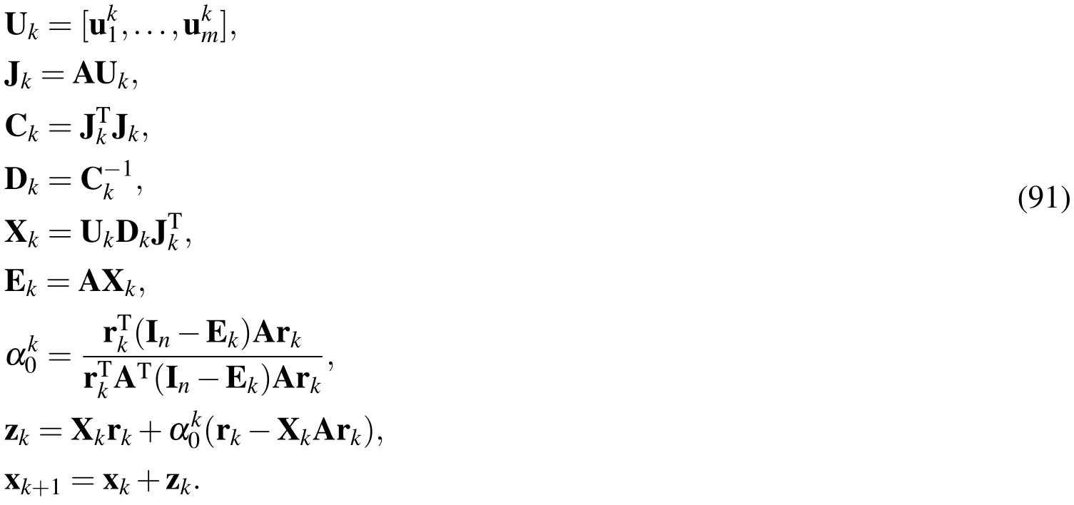
If xk+1converges according to a given stopping criterion ‖rk+1‖ ＜ ε,then stop;otherwise,go to step(ii).

Corollary 2:In the algorithm DOIA,Theorem 3 guarantees that the residual is decreasing step-by-step,of which the residual vectorsrk+1andrkhave the following monotonically decreasing relations:

Proof:For the DOIA,from Eqs.(90)and(85)by taking r=rk+1,r0=rkand y=ykwe have

Inserting Eq.(95)into Eq.(94)we can derive Eq.(92),whereas Eq.(93)follows from Eq.(92)by noting that both Ekand In−Ekare projection operators as shown in Eq.(82).□

Corollary 2 is very important,which guarantees that the algorithm DOIA is absolutely convergent step-by-step with a positive quantity ‖yk‖2＞ 0 being decreased at each iteration step.By using Eqs.(3)and(19),‖yk‖2= ‖Axk−Ax0‖2.

Corollary 3:In the algorithm DOIA,the residual vectorrk+1isA-orthogonal to the descent directionzk,i.e.,

Proof:From r=b−Ax and Eqs.(29)and(19)we have

Taking the inner product with y and using Eq.(87),it follows that

Letting r=rk+1and z=zk,Eq.(96)is proven.□

The DOIA provides a good approximation of the residual Eq.(4)with a better descent direction zkin the affine Krylov subspace.Under this situation we can prove the following corollary.

Corollary 4:In the algorithm DOIA,the residual vectorsrkandrk+1are nearly orthogonal,i.e.,

Moreover,the convergence rate is given by

whereθis the intersection angle betweenrkandy.

Proof:First,in the DOIA,the residual Eq.(4)is approximately satisfied:

Taking the inner product with rk+1and using Eq.(96),Eq.(99)is proven.

Next,from Eqs.(90)and(87)we have

where 0＜θ＜π is the intersection angle between rkand y.Again,with the help of Eq.(87)we also have

Then,Eq.(102)can be further reduced to

Taking the square roots of both sides we can obtain Eq.(100).□

Remark 5:For Eq.(95)in terms of the intersection angle φ between(In−E)rkand(In−E)Arkwe have

If φ =0,for example rkis an eigenvector of A,‖yk‖2= ‖rk‖2can be deduced from Eq.(105)by

Then,by Eq.(94)the DOIA converges with one step more.On the other hand,if we takem=n,then the DOIA also converges with one step.We can see that if a suitable value ofmis taken then the DOIA can converge withinnsteps.Therefore,we can use the following convergence criterion of the DOIA:If

then the iterations in Eq.(91)terminate,whereN≤n.ε1is a given error tolerance.

Theorem 4:The square residual norm obtained by the algorithm which minimizes the merit function(7)in anm-dimensional Krylov subspace is denoted by‖rk+1‖2LS.Then,we have

Proof:The algorithm which minimizes the merit function(7)in anm-dimensional Krylov subspace is a special case of the present theory with α0=0[Liu(2013d)].

Refer Eqs.(8)and(9)as well as Remark 3 for definite.For this case,by Eq.(81)we have

On the other hand,by Eqs.(94)and(95)we have

Subtracting the above two equations we can derive

which by Eq.(82)leads to Eq.(107).□

The algorithm DOIA is better than those algorithms which are based on the minimization in Eq.(7)in anm-dimensional Krylov subspace,including the FOM and GMRES.

5 A double optimal regularization method and algorithm

If A in Eq.(1)is a severely ill-conditioned matrix and the right-hand side data b are disturbanced by a large noise,we may encounter the problem that the numerical solution of Eq.(1)might deviate from the exact one to a great extent.Under this situation we have to solve system(1)by aregularization method.Hansen(1992)and Hansen and O’Leary(1993)have given an illuminating explanation that the Tikhonov regularization method to cope ill-posed linear problem is taking a tradeoff between the size of the regularized solution and the quality to fit the given data by solving the following minimization problem:

In this regularization theory a parameter β needs to be determined[Tikhonov and Arsenin(1977)].

In order to solve Eqs.(1)and(4)we propose a novel regularization method,instead of the Tikhonov regularization method,by minimizing

to find the double optimal regularization solution of z,where y=Az.In Theorem 4 we have proved that the above minimization of the first term is better than that of the minimization of‖r0−Az‖2.

We can derive the following result as an approximate solution of Eq.(112).

Theorem 5:Under the double optimal solution ofz∈given in Theorem 1,an approximate solution of Eq.(112),denoted byZ,is given by

Proof:The first term infin Eq.(112)is scaling invariant,which means that if y is a solution,then γy,γ/=0,is also a solution.Let z be a solution given in Theorem 1,which is a double optimal solution of Eq.(112)with β=0.We suppose that an approximate solution of Eq.(112)with β ＞ 0 is given by Z= γz,where γ is to be determined.

By using Eq.(87),fcan be written as

which upon using Z= γz and y=AZ= γAz becomes

Taking the differential offwith respect to γ and setting the resultant equal to zero we can derive Eq.(113).□

The numerical algorithm based on Theorem 5 is labeled adouble optimal regularization algorithm(DORA),which can be summarized as follows.

(i)Select β,mand give an initial value of x0.

(ii)Fork=0,1,...,we repeat the following computations:

If xk+1converges according to a given stopping criterion ‖rk+1‖ ＜ ε,then stop;otherwise,go to step(ii).It is better to select the value of regularization parameter β in a range such that the value of γkis O(1).We can view γkas a dynamical relaxation factor.

6 Numerical examples

In order to evaluate the performance of the newly developed algorithms DOIA and DORA,we test some linear problems and compare the numerical results with that obtained by the FOM and GMRES.

6.1 Example 1

First we consider Eq.(1)with the following cyclic coefficient matrix:

where the right-hand side of Eq.(1)is supposed to bebi=i2,i=1,...,6.We use the QR method to find the exact solutions ofxi,i=1,...,6,which are plotted in Fig.1 by solid black line.

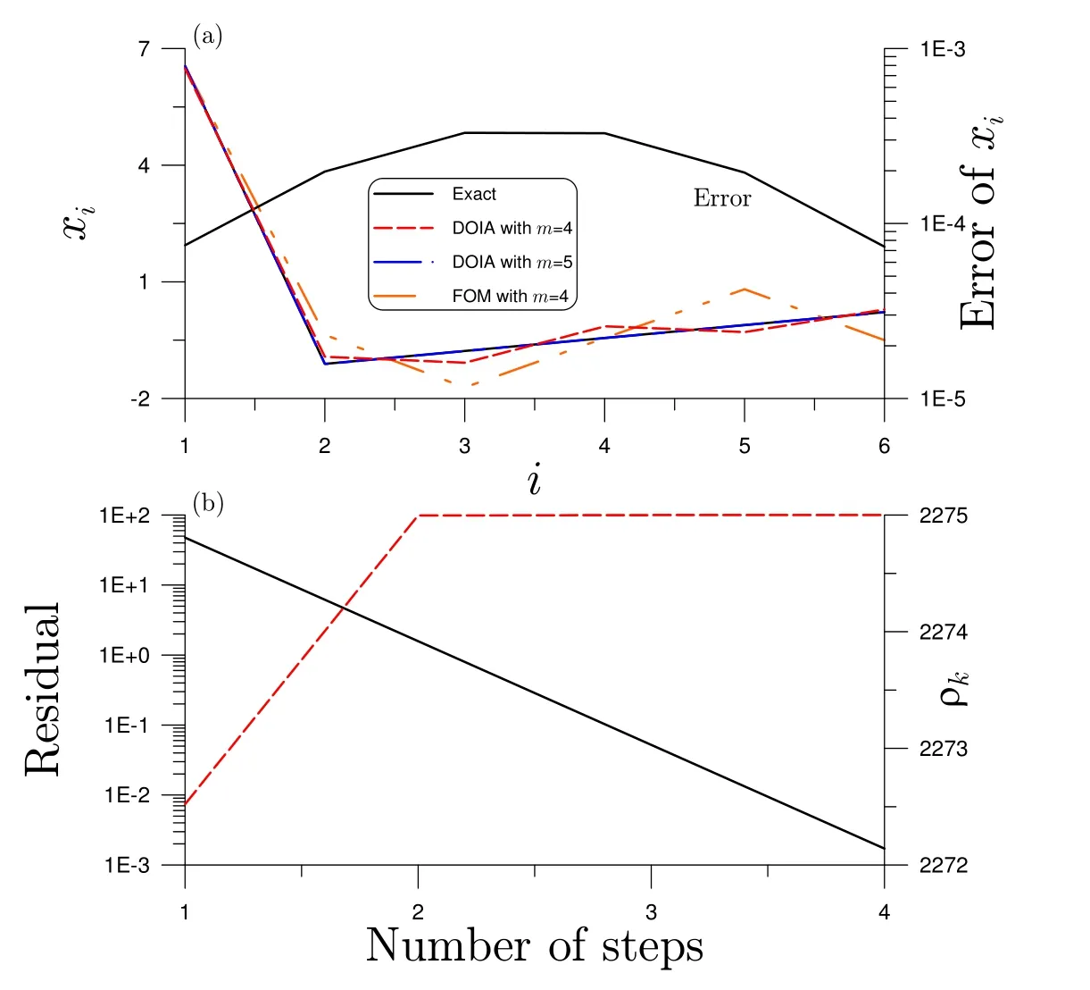
Figure 1:For example 1 solved by optimal solutions of DOIA and FOM,(a)comparing with exact solution and numerical error,and(b)residual and ρk.

In order to evaluate the performance of the DOIA,we use this example to demonstrate the idea of double optimal solution.When we take x0=0 without iterating the solution of z is just the solution x of Eq.(1).We take resrectivelym=4 andm=5 in the DOIA double optimal solutions,which as shown in Fig.1 are close to the exact one.Basically,whenm=5 the double optimal solution is equal to the exact one.We can also see that the double optimal solution withm=4 is already close to the exact one.We apply the same idea to the FOM solution withm=4,which is less accurate than that obtained by the DOIA withm=4.

Now we apply the DOIA under the convergence criterion in Eq.(106)to solve this problem,where we takem=4 and ε1=10−8.With four stepsN=4 we can obtain numerical solution whose error is plotted in Fig.1(a)by solid black line,which is quite accurate with the maximum error being smaller than 3.3×10−4.The residual is plotted in Fig.1(b)by solid black line.The value of square initial residual is‖r0‖2=2275 and the term ρkfast tends to 2275 at the first two steps,and then atN=4 the value of ρNis over‖r0‖2−ε1.

6.2 Example 2

When we apply a central difference scheme to the following two-point boundary value problem:

we can derive a linear equations system:

where ∆x=1/(n+1)is the spatial length,andui=u(i∆x),i=1,...,n,are unknown values ofu(x)at the grid pointsxi=i∆x.u0=aandun+1=bare the given boundary conditions.The above matrix A is known as a central difference matrix,which is a typical sparse matrix.In the applications of FOM,GMRES and DOIA we taken=99 andm=10,of which the condition number of A is about 4052.

The numerical solutions obtained by the FOM,GMRES and DOIA are compared with the exact solution:

The residuals and numerical errors are compared in Figs.2(a)and 2(b),whose maximum errors are the same value 8.32×10−6.Under the convergence criterion with ε=10−10,the FOM converges with 414 steps,the GMRES converges with 379 steps,and the DOIA is convergent with 322 steps.As shown in Fig.2(a)the DOIA is convergent faster than the GMRES and FOM;however,these three algorithms give the numerical solution having the same accuracy.The orthogonalities specified in Eqs.(96)and(99)for the DOIA are plotted in Fig.2(c).

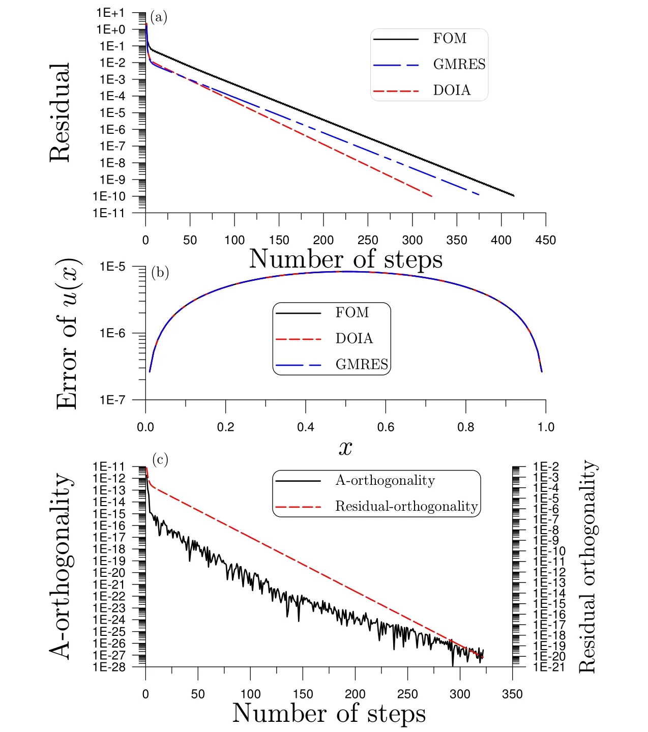
Figure 2:For example 2 solved by the FOM,GMRES and DOIA,comparing(a)residuals,(b)numerical errors,and(c)proving orthogonalities of DOIA.

6.3 Example 3

Finding ann-order polynomial functionp(x)=a0+a1x+...+anxnto best match a continuous functionf(x)in the interval ofx∈[0,1]:

leads to a problem governed by Eq.(1),where A is the(n+1)×(n+1)Hilbert matrix defined by

x is composed of then+1 coefficientsa0,a1,...,anappeared inp(x),and

is uniquely determined by the functionf(x).

The Hilbert matrix is a notorious example of highly ill-conditioned matrices.Eq.(1)with the matrix A having a large condition number usually displays that an arbitrarily small perturbation of data on the right-hand side may lead to an arbitrarily large perturbation to the solution on the left-hand side.

In this example we consider a highly ill-conditioned linear system(1)with A given by Eq.(123).The ill-posedness of Eq.(1)increases fast withn.We consider an exact solution withxj=1,j=1,...,nandbiis given by

whereR(i)are random numbers between[−1,1].

First,a noise with intensity σ =10−6is added on the right-hand side data.Forn=300 we takem=5 for both FOM and DOIA.Under ε=10−3,both FOM and DOIA are convergent with 3 steps.The maximum error obtained by the FOM is 0.037,while that obtained by the DOIA is 0.0144.In Fig.3 we show the numerical results,of which the accuracy of DOIA is good,although the ill-posedness of the linear Hilbert problemn=300 is highly increased.

Then we raise the noise to σ =10−3,of which we find that both the GMRES and DOIA under the above convergence ε=10−3andm=5 lead to failure solutions.So we take ε=10−1for the GMRES,DOIA and DORA,where β =0.00015 is used in the DORA.The GMRES runs two steps as shown in Fig.4(a)by dasheddotted line,and the maximum error as shown in Fig.4(b)by dashed-dotted line is 0.5178.The DOIA also runs with two iterations as shown in Fig.4(a)by dashed line,and the maximum error as shown in Fig.4(b)by dashed line is reduced to 0.1417.It is interesting that although the DORA runs 49 iterations as shown in Fig.4(a)by solid line,the maximum error as shown in Fig.4(b)by solid line is largely reduced to 0.0599.For this highly noised case the DOIA is better than the GMRES,while the DORA is better than the DOIA.It can be seen that the improvement of regularization by the DORA is obvious.

Figure 3:For example 3 solved by the FOM and DOIA,(a)residuals,(b)showing α0,and(c)numerical errors.

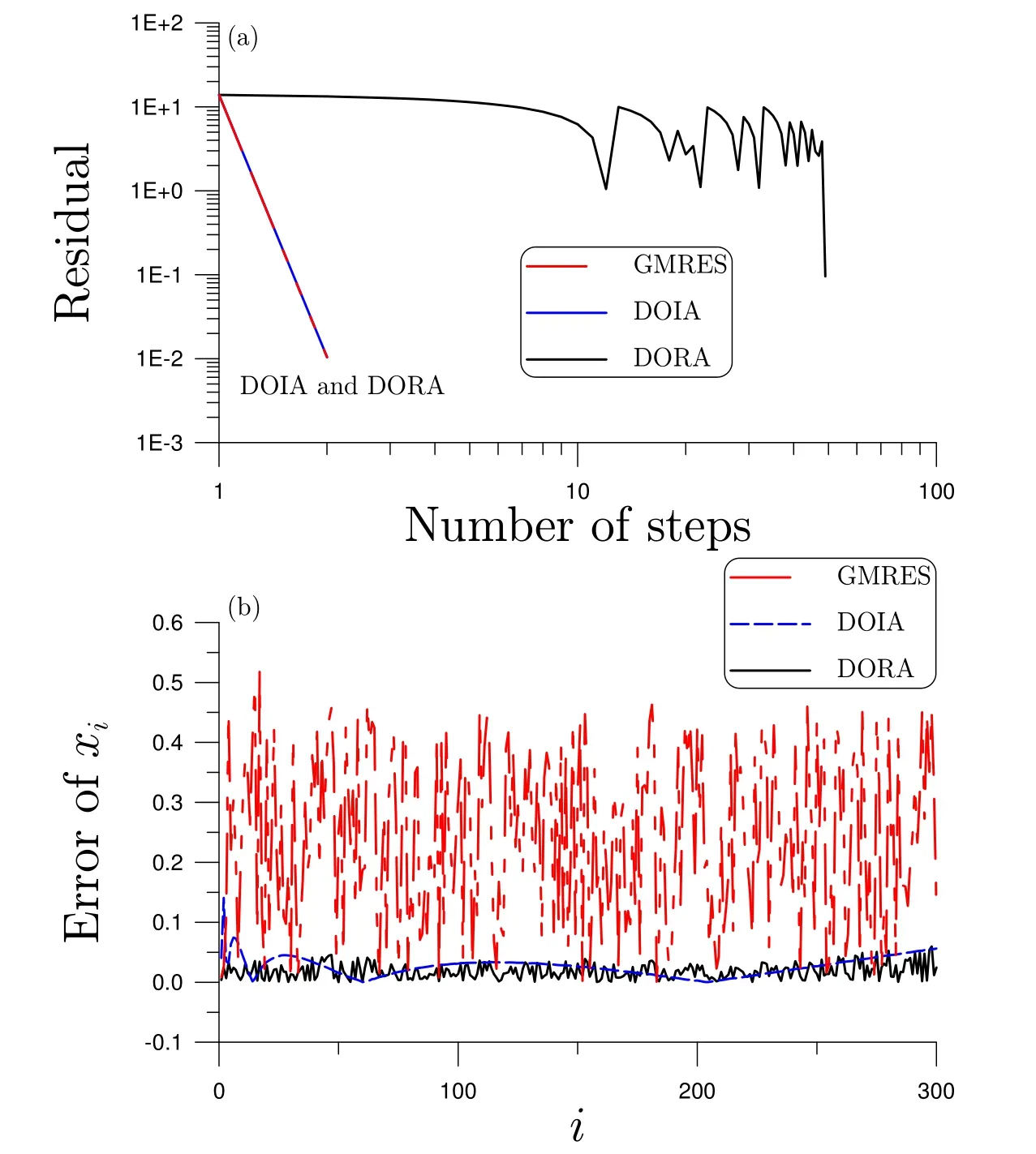
Figure 4:For example 3 under a large noise solved by the GMRES,DOIA and DORA,(a)residuals,and(b)numerical errors.

6.4 Example 4

When the backward heat conduction problem(BHCP)is considered in a spatial interval of 0＜x＜ℓ by subjecting to the boundary conditions at two ends of a slab:

we solveuunder a final time condition:

The fundamental solution of Eq.(126)is by

whereH(t)is the Heaviside function.

In the MFS the solution ofuat the field point p=(x,t)can be expressed as a linear combination of the fundamental solutionsU(p,sj):

wherenis the number of source points,cjare unknown coefficients,and sjare source points being located in the complement Ωcof Ω =[0,ℓ]× [0,T].For the heat conduction equation we have the basis functions

It is known that the location of source points in the MFS has a great influence on the accuracy and stability.In a practical application of MFS to solve the BHCP,the source points are uniformly located on two vertical straight lines parallel to thet-axis,not over the final time,which was adopted by Hon and Li(2009)and Liu(2011),showing a large improvement than the line location of source points below the initial time.After imposing the boundary conditions and the final time condition to Eq.(129)we can obtain a linear equations system(1)with

andn=2m1+m2.

Since the BHCP is highly ill-posed,the ill-condition of the coefficient matrix A in Eq.(1)is serious.To overcome the ill-posedness of Eq.(1)we can use the DOIA and DORA to solve this problem.Here we compare the numerical solution with an exact solution:

For the case withT=1 the value of final time data is in the order of 10−4,which is small by comparing with the value of the initial temperaturef(x)=u0(x)=cos(πx)to be retrieved,which isO(1).First we impose a relative random noise with an intensity σ=10%on the final time data.Under the following parametersm1=15,m2=8,m=16,and ε=10−2,we solve this problem by the FOM,GMRES and DOIA.With two iterations the FOM is convergent as shown Fig.5(a);however,the numerical error as shown in Fig.5(b)is quite large,with the maximum error being 0.264.It means that the FOM is failure for this inverse problem.The DOIA is convergent with five steps,and its maximum error is 0.014,while the GMRES is convergent with 16 steps and with the maximum error being 0.148.It can be seen that the present DOIA converges very fast and is very robust against noise,and we can provide a very accurate numerical result of the BHCP by using the DOIA.

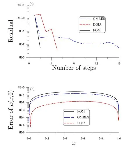
Figure 5:For example 4 solved by the FOM,GMRES and DOIA,comparing(a)residuals,and(b)numerical errors.

Next,we come to a very highly ill-posed case withT=5 and σ=100%.When the final time data are in the order of 10−21,we attempt to recover the initial tempera-turef(x)=cos(πx)which is in the order of 100.Under the following parametersm1=10,m2=8,m=16,and ε=10−4and ε1=10−8,we solve this problem by the DOIA and DORA,where β=0.4 is used in the DORA.We let DOIA and DORA run 100 steps,because they do not converge under the above convegence criterion ε=10−4as shown in Fig.6(a).Due to a large value of β =0.4,the residual curve of DORA is quite different from that of the DOIA.The numerical results ofu(x,0)are compared with the exact onef(x)=cos(πx)in Fig.6(b),whose maximum error of the DOIA is about 0.2786,while that of the DORA is about 0.183.It can be seen that the improvement is obvious.

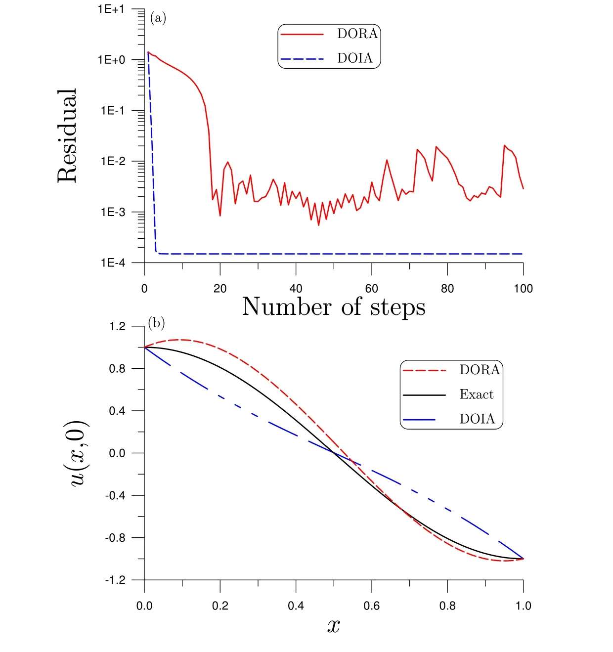
Figure 6:For example 4 under large final time and large noise solved by the DOIA and DORA,comparing(a)residuals,(b)numerical solutions and exact solution,and(c)numerical errors.

6.5 Example 5

Let us consider the inverse Cauchy problem for the Laplace equation:

whereh(θ)andg(θ)are given functions.The inverse Cauchy problem is specified as follows:Seeking an unknown boundary functionf(θ)on the part Γ2:={(r,θ)|r= ρ(θ),π ＜ θ ＜ 2π}of the boundary under Eqs.(132)-(134)with the overspecified data being given on Γ1:={(r,θ)|r= ρ(θ),0 ≤ θ ≤ π}.It is well known that the inverse Cauchy problem is a highly ill-posed problem.In the past,almost all of the checks to the ill-posedness of the inverse Cauchy problem,the illustrating examples have led to that the inverse Cauchy problem is actually severely ill-posed.Belgacem(2007)has provided an answer to the ill-posedness degree of the inverse Cauchy problem by using the theory of kernel operators.The foundation of his proof is the Steklov-Poincaré approach introduced in Belgacem and El Fekih(2005).

The method of fundamental solutions(MFS)can be used to solve the Laplace equation,of which the solution ofuat the field point p=(rcosθ,rsinθ)can be expressed as a linear combination of fundamental solutionsU(p,sj):

For the Laplace equation(132)we have the fundamental solutions:

In the practical application of MFS,by imposing the boundary conditions(133)and(134)atNpoints on Eq.(135)we can obtain a linear equations system(1)with

in whichn=2N,and

The aboveR(θ)=ρ(θ)+Dwith an offsetDcan be used to locate the source points along a contour with a radiusR(θ).

For the purpose of comparison we consider the following exact solution:

defined in a domain with a complex amoeba-like irregular shape as a boundary:

We solve this problem by the DOIA and DORA withn=2N=40 andm=10,where the noise being imposed on the measured datahandgis quite large with σ=0.3,and β=0.0003 is used in the DORA.Through 10 iterations for both the DOIA and DORA the residuals are shown in Fig.7(a).The numerical solutions and exact solution are compared in Fig.7(b).It can be seen that the DOIA and DORA can accurately recover the unknown boundary condition.As shown in Fig.7(c),when the DOIA has the maximum error 0.381,the DORA has the maximum error 0.253.We also apply the GMRES withm=10 to solve this problem;however,as shown in Fig.7 it is failure,whose maximum error is 2.7.

Next we consider a large noise with σ =40%.The value of β used in the DORA is changed to β=0.000095.Through 100 iterations for both the DOIA and DORA the residuals are shown in Fig.8(a).The numerical solutions and exact solution are compared in Fig.8(b).As shown in Fig.8(c),when the DOIA has the maximum error 0.5417,the DORA has the maximum error 0.2737.The improvement of the accuracy by using the DORA than the DOIA is obvious.

Accordingly,we can observe that the algorithms DOIA and DORA can deal with the Cauchy problem of the Laplace equation in a domain with a complex amoebalike irregular shape even under very large noises up to σ =30%and σ =40%,and yield much better results than that obtained by the GMRES.

6.6 Example 6

One famous mesh-less numerical method used in the data interpolation for two dimensional functionu(x,y)is the radial basis function(RBF)method,which expandsuby

Figure 7:For example 5 solved by the GMRES,DOIA and DORA,comparing(a)residuals,(b)numerical solutions and exact solution,and(c)numerical errors.

whereakare the expansion coefficients to be determined and φkis a set of RBFs,for example,

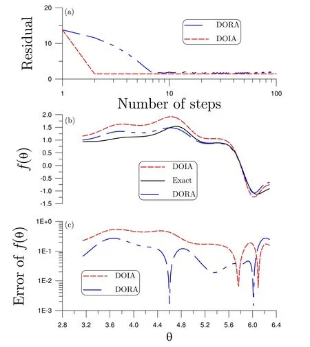
Figure 8:For example 5 under large noise solved by the DOIA and DORA,comparing(a)residuals,(b)numerical solutions and exact solution,and(c)numerical errors.

where the radius functionrkis given byrk=whilek=1,...,nare called source points.The constantsaandcare shape parameters.In the below we take the first set of φkas trial functions,withN=2 which is known as a multi-quadric RBF[Golberg and Chen(1996);Cheng,Golberg and Kansa(2003)].There are some discussions about the optimal shape factorcused in the MQ-RBF[Huang,Lee and Cheng(2007);Huang,Yen and Cheng(2010);Bayona,Moscoso and Kindelan(2011);andCheng(2012)].

We solve a quite difficult and well known interpolation problem of Franke function[Franke(1982)]:

on the unit square.We apply the DOIA withm=5 andc=0.3 to solve this problem under the convergence criterion ε=0.1,where we take∆x= ∆y=1/9 to be a uniform spacing of distribution of source points as that used in Fasshauer(2002).The residual is shown in Fig.9(a),which is convergent with 22 iterations,and the numerical error is shown in Fig.9(b).The maximum error 0.0576 obtained by the DOIA is better than 0.1556 obtained by Fasshauer(2002).

7 Conclusions

In an affinem-dimensional Krylov subspace we have derived a closed-form double optimal solution of then-dimensional linear residual equation(4),which was obtained by optimizing two merit functions in Eqs.(27)and(30).The main properties were analyzed,and a key equation was proven to link these two optimizations.Based on the double optimal solution,the iterative algorithm DOIA was developed,which has an A-orthogonal property, and is proven to be absolutely convergent step by-step with the square residual error being reduced by a positive quantity ‖Azk‖2at each iteration step.We have proved that the residual error obtained by the algorithm DOIA is smaller than that obtained by other algorithms which are based on the minimization of the square residual error‖b−Ax‖2,including the FOM and GMRES.We developed as well a simple double optimal regularization algorithm(DORA)to tackle the ill-posed linear problem under a large noise,and as compared with the GMRES and DOIA the regularization effect obtained by the DORA is obvious.Because the computational costs of DOIA and DORA are very inexpensive with the need of only inverting anm×mmatrix one time at each iterative step,they are very useful to solve a large scale system of linear equations with an ill-conditioned coefficient matrix.Even when we imposed a large noise on the ill-posed linear inverse problem,the DOIA and DORA were robust against large noise,but both the FOM and GMRES were not workable.

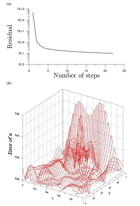
Figure 9:For the data interpolation of Franke function,showing(a)residual,and(b)numerical error computed by the DOIA.

Acknowledgement:Highly appreciated are the project NSC-102-2221-E-002-125-MY3 and the 2011 Outstanding Research Award from the National Science Council of Taiwan to the first author.The work of the second author is supported by a UCI/ARL coll oborative research grant.

Bayona,V.;Moscoso,M.;Kindelan,M.(2011):Optimal constant shape parameter for multiquadric based RBF-FD method.J.Comput.Phys.,vol.230,pp.7384-7399.

Ben Belgacem,F.(2007):Why is the Cauchy problem severely ill-posed?Inverse Problems,vol.23,pp.823-836.

Ben Belgacem,F.;El Fekih,H.(2005):On Cauchy’s problem:I.A variational Steklov-Poincaré theory.Inverse Problems,vol.21,pp.1915-1936.

Cheng,A.H.D.(2012):Multiquadric and its shape parameter–A numerical investigation of error estimate,condition number,and round-off error by arbitrary precision computation.Eng.Anal.Bound.Elem.,vol.36,pp.220-239.

Cheng,A.H.D.;Golberg,M.A.;Kansa,E.J.;Zammito,G.(2003):Exponential convergence and H-c multiquadric collocation method for partial differential equations.Numer.Meth.Par.Diff.Eqs.,vol.19,pp.571-594.

Daubechies,I.;Defrise,M.;De Mol,C.(2004):An iterative thresholding algorithm for linear inverse problems with a sparsity constraint.Commun.Pure Appl.Math.,vol.57,pp.1413-1457.

Dongarra,J.;Sullivan,F.(2000):Guest editors’introduction to the top 10 algorithms.Comput.Sci.Eng.,vol.2,pp.22-23.

Fasshauer,G.E.(2002):Newton iteration with multiquadrics for the solution of nonlinear PDEs.Comput.Math.Appl.,vol.43,pp.423-438.

Fletcher,R.(1976):Conjugate gradient methods for indefinite systems.Lecture Notes in Math.,vol.506,pp.73-89,Springer-Verlag,Berlin.

Franke,R.(1982):Scattered data interpolation:tests of some method.Math.Comput.,vol.38,pp.181-200.

Freund,R.W.;Nachtigal,N.M.(1991):QMR:a quasi-minimal residual method for non-Hermitian linear systems.Numer.Math.,vol.60,pp.315-339.

Golberg,M.A.;Chen,C.S.;Karur,S.R.(1996):Improved multiquadric approximation for partial differential equations.Eng.Anal.Bound.Elem.,vol.18,pp.9-17.

Hansen,P.C.(1992):Analysis of discrete ill-posed problems by means of the L-curve.SIAM Rev.,vol.34,pp.561-580.

Hansen,P.C.;O’Leary,D.P.(1993):The use of the L-curve in the regularization of discrete ill-posed problems.SIAM J.Sci.Comput.,vol.14,pp.1487-1503.

Hestenes,M.R.;Stiefel,E.L.(1952):Methods of conjugate gradients for solving linear systems.J.Res.Nat.Bur.Stand.,vol.49,pp.409-436.

Hon,Y.C.;Li,M.(2009):A discrepancy principle for the source points location in using the MFS for solving the BHCP.Int.J.Comput.Meth.,vol.6,pp.181-197.

Huang,C.S.;Lee,C.F.;Cheng,A.H.D.(2007):Error estimate,optimal shape factor,and high precision computation of multiquadric collocation method.Eng.Anal.Bound.Elem.,vol.31,pp.614-623.

Huang,C.S.;Yen,H.D.;Cheng,A.H.D.(2010):On the increasingly flat radial basis function and optimal shape parameter for the solution of elliptic PDEs.Eng.Anal.Bound.Elem.,vol.34,pp.802-809.

Lanczos,C.(1952):Solution of systems of linear equations by minimized iterations.J.Res.Nat.Bur.Stand.,vol.49,pp.33-53.

Liu,C.-S.(2011):The method of fundamental solutions for solving the backward heat conduction problem with conditioning by a new post-conditioner.Numer.Heat Transf.B:Fund.,vol.60,pp.57-72.

Liu,C.-S.(2012a):The concept of best vector used to solve ill-posed linear inverse problems.CMES:Computer Modeling in Engineering&Sciences,vol.83,pp.499-525.

Liu,C.-S.(2012b):A globally optimal iterative algorithm to solve an ill-posed linear system,CMES:Computer Modeling in Engineering&Sciences,vol.84,pp.383-403.

Liu,C.-S.(2013a):An optimal multi-vector iterative algorithm in a Krylov subspace for solving the ill-posed linear inverse problems.CMC:Computers,Materials&Continua,vol.33,pp.175-198.

Liu,C.-S.(2013b):An optimal tri-vector iterative algorithm for solving ill-posed linear inverse problems.Inv.Prob.Sci.Eng.,vol.21,pp.650-681.

Liu,C.-S.(2013c):A dynamical Tikhonov regularization for solving ill-posed linear algebraic systems.Acta Appl.Math.,vol.123,pp.285-307.

Liu,C.-S.(2013d):Discussing a more fundamental concept than the minimal residual method for solving linear system in a Krylov subspace.J.Math.Research,vol.5,pp.58-70.

Liu,C.-S.(2014a):A doubly optimized solution of linear equations system expressed in an affine Krylov subspace.J.Comput.Appl.Math.,vol.260,pp.375-394.

Liu,C.-S.(2014b):A maximal projection solution of ill-posed linear system in a column subspace,better than the least squares solution.Comput.Math.Appl.,vol.67,pp.1998-2014.

Liu,C.-S.(2014c):Optimal algorithms in a Krylov subspace for solving linear inverse problems by MFS.Eng.Anal.Bound.Elem.,vol.44,pp.64-75.

Liu,C.-S.(2015):A double optimal descent algorithm for iteratively solving illposed linear inverse problems.Inv.Prob.Sci.Eng.,vol.23,pp.38-66.

Matinfar,M.;Zareamoghaddam,H.;Eslami,M.;Saeidy,M.(2012):GMRES implementations and residual smoothing techniques for solving ill-posed linear systems.Comput.Math.Appl.,vol.63,pp.1-13.

Paige,C.C.;Saunders,M.A.(1975):Solution of sparse indefinite systems of linear equations.SIAM J.Numer.Ana.,vol.12,pp.617-629.

Saad,Y.(1981):Krylov subspace methods for solving large unsymmetric linear systems.Math.Comput.,vol.37,pp.105-126.

Saad,Y.(2003):Iterative Methods for Sparse Linear Systems.2nd Ed.,SIAM,Pennsylvania.

Saad,Y.;Schultz,M.H.(1986):GMRES:A generalized minimal residual algorithm for solving nonsymmetric linear systems.SIAM J.Sci.Stat.Comput.,vol.7,pp.856-869.

Saad,Y.;van der Vorst,H.A.(2000):Iterative solution of linear systems in the 20th century.J.Comput.Appl.Math.,vol.123,pp.1-33.

Simoncini,V.;Szyld,D.B.(2007):Recent computational developments in Krylov subspace methods for linear systems.Numer.Linear Algebra Appl.,vol.14,pp.1-59.

Sonneveld,P.(1989):CGS:a fast Lanczos-type solver for nonsymmetric linear systems.SIAM J.Sci.Stat.Comput.,vol.10,pp.36-52.

Tikhonov,A.N.;Arsenin,V.Y.(1977):Solutions of Ill-Posed Problems.John-Wiley&Sons,New York.

van Den Eshof,J.;Sleijpen,G.L.G.(2004):Inexact Krylov subspace methods for linear systems.SIAM J.Matrix Anal.Appl.,vol.26,pp.125-153.

van der Vorst,H.A.(1992):Bi-CGSTAB:a fast and smoothly converging variant of Bi-CG for the solution of nonsymmetric linear systems.SIAM J.Sci.Stat.Comput.,vol.13,pp.631-644.

van der Vorst,H.A.(2003):Iterative Krylov Methods for Large Linear Systems.Cambridge University Press,New York.

1Department of Civil Engineering,National Taiwan University,Taipei,Taiwan. E-mail:liucs@ntu.edu.tw

2Center for Aerospace Research&Education,University of California,Irvine.