Least Squares Stochastic Finite Element Method in Structural Stability Analysis of Steel Skeletal Structures1

Marcin Kami´nskiand Jacek Szafran

Least Squares Stochastic Finite Element Method in Structural Stability Analysis of Steel Skeletal Structures1

Marcin Kami´nski2and Jacek Szafran3

Basic probabilistic characteristics and reliability indices of critical forces for high steel skeletal towers are numerically modeled by using the Stochastic,perturbation-based Finite Element Method.It is implemented together with the Weighted Least Squares Method and compared with the Monte-Carlo simulation as well as with the semi-analytical Probabilistic FEM.The Finite Element Method solution to the stability problem for a full 3D model of a tower accounts for both first and second order effects known from the engineering codes as the so-called P-delta effect.Two different Gaussian input random variables are adopted here–Young modulus of steel as well as principal structural elements thickness–to compare an influence of the material versus the geometrical uncertainty on the overall structural response.The numerical analysis has been carried out with a combination of the FEM engineering program with symbolic algebra software providing WLSM approximation,probabilistic simulation,integration,as well as for the general order Taylor expansion procedures.The reliability indices related to the stability problem are calculated using both the First and the Second Order Reliability Methods and they showed safety margins for the telecommunication towers.

Least Squares Method;Stochastic Finite Element Method;generalized stochastic perturbation technique;stability problems;steel skeletal structures;semi-analytical method;Monte-Carlo simulation

1 Introduction

Designing of spatial large scale skeletal structures frequently needs an extra upgrade of technological equipment,sometimes apparently beyond the design limits given in the initial structural project. There is no doubt that this needs geometrically nonlinear Finite Element Method(FEM)analysis,frequently towards the structural stability modeling.A veri fication of the capacity margin must be complemented each time with such a stability analysis taking into consideration both global as well as local imperfections and instabilities as far as the steel(or aluminum)thinwalled structures are considered.Computational analysis,provided within the use of the FEM or some of its stochastic counterparts,should account for all the external loads,where the technological one is adjacent to the incrementation procedure,leading to a determination of the critical load multipliers.It is usually done accounting for the buckling FEM analysis,where constitutive,initial stress and initial displacements stiffness matrices compose the overall engineering structure stiffness.On the other hand,the uncertainty sources are introduced in the form of various geometrical imperfections,stochastic losses of a given cross-section due to corrosion process[Melchers(1987);Sadovský and Drdácký(2001)],environmental external loadings relevant to accidental ice covers,additional wind pressures or even to unpredictable fire exposure.They all in fluence the non-dimensional reliability index that can be calculated according to the First(FORM)or the Second Order Reliability Methods(SORM),where the stress limit function is traditionally de fined as a difference in-between computed normal stresses and adjacent critical stresses.Some other issues connected with uncertainty analysis corresponding to the stability analysis may be found in[Elishakoff(1983);Elishakoff,Li and Starnes(2001)].Stochastic analyses that are necessary for further reliability determination are widely used in many branches of civil engineering research articles,e.g.[Hosseini,Shahabian,Sladek and Sladek(2011);Lin,Liu,Yuan and Mang(2014);Silva,Azikri de Deus,Mantovani and Beck(2010);Yang,Li and Cai(2013)].

The main purpose of this work is to apply the Least Squares Method(initsweighted extended version)in the higher order perturbation-based Stochastic Finite Element Method[Kami´nski(2013);Kami´nski and Solecka(2013);Kami´nski and Str˛akowski(2013)]developed through an extension of the Second Order Second Moment(SOSM)stochastic perturbation approach[Kleiber,and Hien(1992)].Another goal is to contrast the resulting basic probabilistic characteristics with these computed with the semi-analytical approach and,independently,with these estimated via the classical Monte-Carlo simulation scheme.Semi-analytical method uses the same response functions resulting from the LSM procedure as stochastic perturbation technique,however further determination of the probabilistic characteristics for the state functions proceeds through symbolic integration according to the ba-sic de finition of the probability theory.Particularly,we demonstrate an application of our triple probabilistic computational strategy to stability analysis of the steel lattice towers to verify an opportunity to upgrade them significantly beyond initial designing limits in presence of some structural random parameters.Computational stability verification is provided here according to both the first and the second order reliability theories.Such a study has been carried out here for the specific steel telecommunication tower having randomized Young modulus and,independently,for the mean thickness of the tower legs made with using round seamless pipes statistically dispersed according to the Gaussian probability distribution function.We de fine here the critical load as a multiplier of the unit vectors located at the tower top and acting downwards;it simulates the capacity margin for this structure accounting for the extra equipment to be mounted at its top during further exploitation.Probabilistic computational analysis is focused on statistical and probabilistic determination of the expected values,coefficients of variation,skewness and kurtosis of the critical load multipliers.We examine probabilistic convergence of all the aforementioned characteristics together with the order of stochastic perturbation applied and with respect to the input coefficient of variation belonging to the intervalα∈[0.00,0.15].Finally,we verify also whether the critical load magnitude is the Gaussian variable to conditionally apply the simplified reliability index formula that consists of a ratio of the expectation to the standard deviation of the proposed limit function.Such a reliability index calculated according to the Cornell theory[Melchers(1987)],treated as equivalent to the First Order Reliability Method(FORM),has been further contrasted here with that calculated according to the Second Order Reliability Method(SORM)as we expect some non-Gaussian stochastic structural response;some other issues and aspects of reliability can be found in works[Huang,Aliabadi and Sharif Kodei(2014);Wang,Gao,Yang and Song(2011)].

The key result in a deterministic context is that such towers,designed rather optimally according to the widely known stress and deformation limit states,have remarkable additional capacity,at least in terms of structural stability,while the extra telecommunication equipment is getting attached.The basic probabilistic research finding is that Gaussian Young modulus induces also Gaussian critical forces in these structures,which seems reasonable taking into account the fundamental Euler formula[Timoshenko and Gere(1961)]widely used in various steel structures[Kamin´ski and Solecka(2013);Kamin´ski and Stra˛kowski(2013)].The stability limits were proven to have apparently non-Gaussian probability distributions while randomizing local element thicknesses.All three probabilistic numerical methods implemented and applied in this study return remarkably consistent results in the given interval of input uncertainty.The very interesting observation is that three different probabilistic techniques applied to the nonlinear elastic analysis return here similar results from both qualitative and even quantitative point of view and some further improvements of the Response Function Method may improve this tendency.

2 Governing variational equations

Let us consider a statistically homogeneous and bounded regionwith no initial stresses or strains having external boundaries∂Ωσand∂Ωu,where the stress and displacement boundary conditions are de fined,respectively.The incremental form of isotropic linear elasticity equilibrium problem of Ω is proposed as

fori,j,k,l=1,2,3.In above equations we denoteρas mass density,∆t¯k-as the vector of boundary forces,δikis the Kronecker delta here,νstands for the Poisson ratio,eserves as Young modulus,∆fkdenotes the increments of the mass forces vector,and traditionally,Cijklis traditionally the elasticity tensor.This problem is solved for the displacement vector increments∆uk(x),the strain tensor increments∆εkl(x),and the stress tensor increments∆σkl(x).We introduce here the tensors∆σkl(x),∆(x)as the first and the second Piola-Kirchhoff stress tensors

The following functional de fined with respect to∆ukis usually introduced[Kleiber(1985)]in order to obtain the additional variational formulation:

whereJ(∆uk)is potential energy functional.Its minimization with respect to ∆uklead to the Finite Element Method(FEM)equations described in the next section.Alternatively,one may apply hybrid formulation of the FEM based on the stress functions.

3 Stochastic Finite Element Method equations

3.1 Stability problem matrix equations

The following well known discretization of the displacement function increments in the RFM analysis[Kami´nski(2013)]is adopted in the SFEM approach:

where:ϕαβis the shape function matrix,∆qβis the vector of increments of the generalized displacements,D(p)βare the unknown coefficients in the Least Squares Method polynomial approximations[Björck(1996);Kami´nski(2013)],bdenotes here the given input random variable andNis the total number of degrees of freedom in the FEM model.Additionally,we propose the following strain tensor components discretization:

One may obtain the functional given above in eqn(9)by inserting these representations into the geometrical and constitutive equations as[Kleiber(1985)]

where the first,the second and the third order stiffness matrices are given as

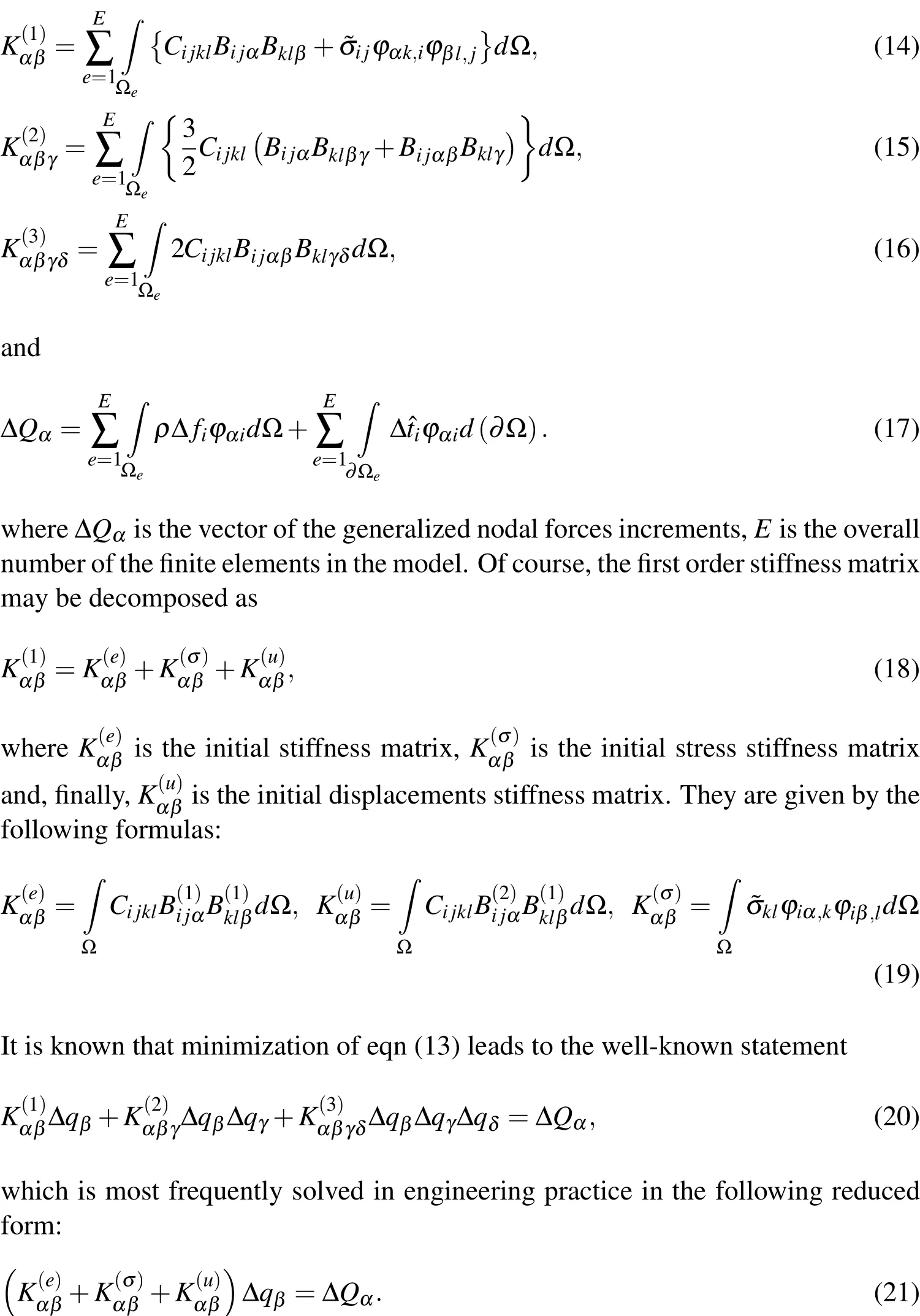
We solve numerically the linearized stability problem given by the matrix equation[Kleiber and Hien(1997)]

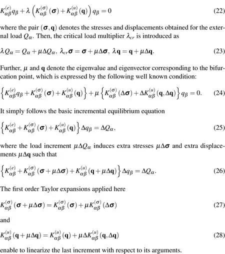
3.2 The Weighted Least Squares Method

Traditionally,the Least Squares Method needs an iterative solution of the initial equilibrium equation(fori=1,...,n)about the expectation of the given input random parameter.This can be applied to our problem in the following manner:

where α,β =1,...,N and λ(i)is the ithcritical load multiplier.It results in a sequenceof the pairsthat enable to recover the polynomial response function for the critical load multiplier as[Kami´nski(2013)]

leading through the generalized stochastic perturbation technique to the fourth order probabilistic characteristics(expectations,coefficients of variation,skewnesses and kurtosis)of this multiplier.Computer analysis obeys here three different cases to distinguish in-between various physical situations– first we postpone last two stiffness matrices in eqn(29)(accounting for the elastic stiffness contribution only),then we make the last matrix negligible,and finally,we solve eqn(29)in its full form.We consider for this purpose a residual in the given trial point indexed by i as a difference between the given critical value and its counterpart coming from the approximating polynomial to be determined f?bi,D(i)?(calculated both for the argument bi).There holds[Björck(1996)]

Computational determination of the coefficients D(i)in this polynomial proceeds from the following gradient equations to minimize the residuals with respect to the coefficients:

We modify this approach by the Aitken weighting procedure[Björck(1996);Kami´nski(2013)],where each trial point is associated to some parameter wii(vector of the weights in WLSM)such that the initial LSM functional equals to

Then,the WLSM gradient,similarly to eqn(33),becomes

Finally,the linear equations system to be solved numerically is rewritten as

All mathematical details of both non-weighted and weighted versions of the LSM technique with additional derivations may be found in[Björck(1996)].

3.3 Determination of the basic probabilistic characteristics

The final probabilistic procedure consists in symbolic calculation of probabilistic moments and coefficients of the critical load multiplier.It proceeds by using of the general order Taylor expansion of this multiplier λcrwith respect to the input Young modulus e[Kami´nski(2013);Kami´nski and Solecka(2013);Kami´nski and Szafran(2012);Sokoł owski,Kami´nski and Str˛akowski(2014)]:

where the order n is smaller than the polynomial order provided in eqn(30)and ε denotes the perturbation parameter;the very similar expansion has been provided independently with respect to the random thickness here.Such an expansion has been further inserted into the equations for the basic probabilistic moments and characteristics of limit λcritself.We show as an illustration the expected values E[λcr]only;there holds

where pe(x)is the probability density function of Young modulus andis the mean value of the critical load multiplier.One may insert ε=1[Kami´nski(2013);Kleiber and Hien(1992)]and to simplify this formula by using of the de finitions of the central probabilistic moments of the Gaussian variable e

where all the moments of an odd order simply vanish here

The same equations are valid in case of the random thickness,whereeis simply replaced withtabove.Moreover,analogous perturbation-based formulas for higher probabilistic moments and coefficients may be derived from the statements included in[Kami´nski(2013);Kami´nski and Solecka(2013);Kami´nski and Szafran(2012);Sokoł owski,Kami´nski and Str˛akowski(2014)].We compare the perturbation-based moments against these calculated by straightforward probabilistic integration of the WLSM-based response functions and,independently,with the Monte-Carlo simulation estimators.Such a classical statistical estimator of the expectation employed in our Monte-Carlo simulation scheme corresponding to the definition(39)is given as

whereb∈{e,t},while the variancesVar(λcr)and thekthcentral probabilistic momentsµk(λcr)are estimated as

Finally,we proceed with determination of the reliability measures.The reliability index calculated according to the First Order Reliability Method,namelyβFORM,assumes Gaussian probability distribution of the given structural response function.The Second Order Reliability Method(SORM)shall be applied in case of the non-Gaussian response.The general formula to calculateβSORMis the following one:

wherePf2denotes the probability of failure for the chosen probability distribution Φ of the function related toβFORMin the following manner:

where κ is curvature of the limit function g(surface)usually de fined as

The formulas given above allow to calculate the reliability indices for arbitrary probability density function describing the critical load multiplier.

4 Computational experiments

We model a steel telecommunication tower[Kami´nski and Szafran(2012)]with the height of 60.0 meters consisting of ten sections,made of steel S355 and having four legs(rectangular horizontal cross-section).It has a linear geometrical convergence up to the ninth segment(at the level of 54.0 meters)and forms a prism with the dimensions 4.82 m×4.82 m at the base and 0.90 m×0.90 m at its top.The basic structural elements are the legs and the diagonal bracing members.The joints between the legs and these braces are made with the bearing type bolts(one per a joint)in lower seven sections and welded in the remaining top segments.Numerical analysis has been entirely conducted using a combination of the structural analysis FEM system ROBOT and the computer algebra system MAPLE.The FEM discretization has been prepared with the use of 400 two-noded elastic truss 3D elements and of 228 two-noded elastic 3D beam elements connected at 806 nodal points(6 DOFs each).The tower legs are modeled here as round structural seamless tubes with diameters ranging from/0 139.7 mm×8 mm to/0 60.3 mm×3 mm;the diagonal bracing members are attached as the cold formed C-bars(lower four sections),seamless tubes(the sections in the middle of the tower)and full round rods at the remaining upper segments.The diagonal bracing members are distributed according to the X pattern for seven lower sections and in K pattern–for the top three segments.The detailed specification of the steel pro files and bolted connections is given in Tab.1 below,while their spatial distribution and the photos are given in Fig.1.

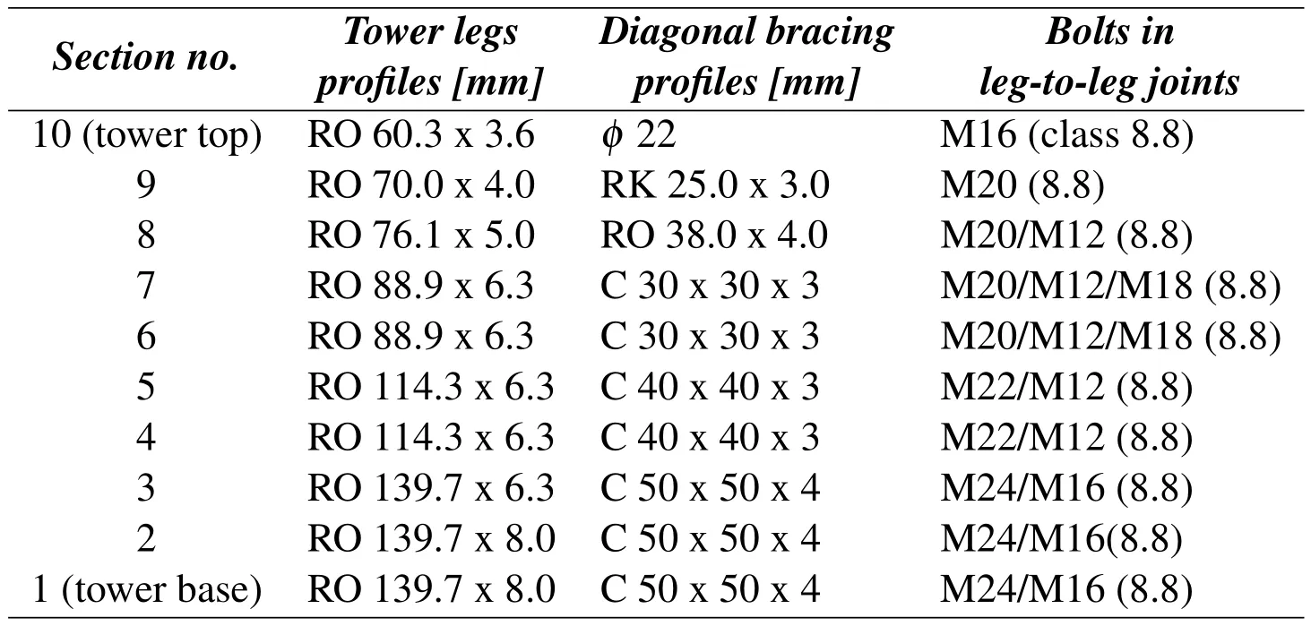
Table 1:Structural steel pro files and connections in the telecommunication tower

We have inserted additionally a steel ring with external diameter equal to 3.47 m located at the level of 55.2 m above the foundation(as visible in Fig.1),where two sector antennas cantilevers(about 1350 mm long)have been attached.We account here for the dead loads,technological installation weight,as well as the wind pressure,while the critical load multiplier is adjacent to the four unit concentrated forces acting downwards and distributed symmetrically on the top steel ring for the antennas cantilevers.

Figure 1:Photo of the existing structure,scheme of th tower,joints between legs and diagonal bracing and discretization of the entire structure in the FEM system ROBOT

Computational analysis consists of the eleven trial points to recover the polynomial response functions relating the critical load multipliers and Young moduluse.These eleven trials in case ofeare:189.0,193.2,197.4,201.6,205.8,210.0,214.2,218.4,222.6,226.8,231.0 GPa(global uncertainty).The corresponding tests with random thicknesstof the legs round tubes thickness(local uncertainty)have been performed for 3.8,4.3,4.8,5.3,5.8,6.3,6.8,7.3,7.8,8.3 and 8.8 mm,respectively.The Finite Element Method analysis obeys the following two cases:(a)initial stiffness matrix(composed using the elastic part only)marked here with the First Order Theory(FOT)and,independently,(b)including extra stiffness fluctuation resulting from the longitudinal forces on the deformed elements marked as Second Order Theory(SOT).We look for three different critical values of the examined engineering structure denoted here as 1st:adjacent to the stability loss by the upper diagonal bracing,13th:corresponding to the stability loss by the legs in bending and, finally,19th:equivalent to the combined twisting-bending mode.Numerical FEM analysis of the tower stability has been carried out using 5 load increments,40 iterations for each load increment,maximum 3 reductions of a single increment,for the coef ficient of the increment length taken as 0.5,and a tolerance of the residual forces equal to 0.0001;the subspace iteration algorithm serves for the deterministic computational solution.We collect the expected values of the 1st(Fig.2),13th(Fig.3)and 19th(Fig.4)critical values according to the first order theory while randomizing Young modulus(left series)and,separately,for random thickness of the tubular legs(right series).All the expectations are consecutively computed according to the 2nd,4th and 6th order stochastic perturbation technique and are all contrasted with the Monte-Carlo simulation results(obtained for M=105random trials)and the semi-analytical symbolic integration of the polynomial responses.Further,we repeat this computational process for the critical forces expectations calculated according to the Second Order Theory(Figs.5–7),in exactly the same arrangement related to the critical value number and to both input random variables.Then,we include the coef ficients of variation(CoV)given accordingly for the First(Figs.8–10)and Second Order(Figs.11–13)theories,skewness(Figs.14–16 in case ofFOTand Figs.17-19 related toSOT),kurtosis(Figs.20–22 –FOTand Figs.23–25 –SOT).Higher order statistics are calculated of course with the use of higher order perturbation orders including most frequently applied tenth order expansion terms[Kami´nski(2013)].They are all given as the functions of the input coefficients of variationα(e)andα(t)belonging to the interval[0.00,0.15]for both random inputs.Such an interval corresponds to the corroded tubes rather than to the Young modulus experimental statistics giving usually two times smaller variability.Computational results are completed with the reliability index exposed in the same manner:with respect to the first(Figs.26–28)and second order(Figs.29–31)theories,but now additionally given for the First Order Reliability Method(FORM)and,for comparison,according to the Second Order Reliability Method(SORM);they are both based on the highest order stochastic perturbation analysis.These results are extended with respect to the basic probabilistic characteristics as the horizontal axis for the input random fluctuations is adjacent to[0.00,0.25],for further possible exploitation during the time-dependent durability veri fication.We postpone the response function recovery in this presentation,because the critical value is almost linearly varying upon the Young modulus(expressed also in the Euler formula and even in Engesser-von Karman theory).These critical values are inversely proportional to the basic structural elements thickness and this proportionality has been recovered via the WLSM calculations also as almost linear relation;these observations are not affected in any way by the stability theory order.

First,we discuss the expected values for the First(Figs.2–4)and the Second(Figs.5–7)Order stability theories–the left series corresponded to random Young modulus and included the 1st,13thand 19thcritical values,while the right one included analogous critical values for random thicknesst.It is characteristic,after comparison between the left and right series graphs,that particular expectations obtained with randomeand,separately,for the geometrical uncertaintytare almost equal to each other;this is not the case of higher order probabilistic characteristics(see Figs.8–25).Contrasted probabilistic methods including various orders stochastic perturbation techniques return almost the same expectations for all the critical forces while randomizing structural thicknesst.Some negligible divergence inbetween these methods has been observed for larger input coefficients of variation in case of the 19thcritical value,but even these extreme differences could be neglected(a range of 1%and less).First critical value increases significantly together with the input stochastic fluctuations,while the other two critical values decrease and the additional expectation fluctuations are curvilinear with constant convexity and with no local oscillations.The results obtained for the Second Order Theory,while randomizingt,are very close to the First Order critical forces,while their variations remain exactly the same.It is also apparent here that the minimum capacity in the view of structural stability is in its upper braces as the ratio of the 1stto the 13thcritical value(when the legs may lose their stability for the first time)equals 3.A situation with the expectations of the three given critical values appears to be more complex while randomizing steel Young modulus.Initially,these expectations all look insensitive to the input coefficient of variation and both stability theories and probabilistic methods return exactly the same results.This happens for the input coefficient of variation in lower range,i.e.α(e)∈[0.00,0.10].The tendencies for all numerical methods out of this interval become highly nonlinear and start to diverge from each other.These differences could be neglected for the First Order Theory but may also have remarkable values,especially in Figs.6 and 7(left column).We need to mention that various order stochastic perturbation methods also return different expectations of the critical values.Nevertheless,it is noticeable that the highest,6th order perturbation technique series is the closest one to the results returned via the semi-analytical method.The Monte-Carlo simulation follows this principal trend for the first order stability analysis,where all the differences are really small,also in case of the 1stcritical value in the second order theory.Summing up,determination of the expected values of critical forces for both material and geometrical uncertainty in the range of input CoV adjacent to the existing experimental evidence may be carried out with almost the same precision by any of the probabilistic methods applied here.

Further,we analyze the coefficients of variation–these resulting from random Young modulus almost all depend linearly upon the input CoV.We add for this purpose the new extra higher order stochastic perturbation technique,because the second order characteristics usually demand larger computational effort than the expectations.We notice a direct proportionality as far as the first order theory has been considered;the output CoV is equal to the input one and all probabilistic methods return exactly the same values.This fact reflects exactly a consequence of the linear transform of the Gaussian random input into the critical force represented by Euler formula.The second order theory results collected in left series of Figs.11–13 are different according to the uncontrolled growth of this CoV computed via semi-analytical technique forα(e)close to 0.15,especially for higher critical values.The diagrams ofα(λ13)andα(λ19)show both rather marginal differences in-between various stochastic perturbation method orders.Therefore,the output uncertainty basically does not depend on the order of the stability method;however,it is strongly related to a choice of the random input type.The right series of graphs in Figs.8–10aswellasFigs.11–13document essentially different tendency for geometrical uncertainty.The output CoV is the few times smaller than the input one,all probabilistic methods return the same linear and direct proportionality for the first critical value only.All these results do not depend upon the stability theory order,but higher critical values demonstrate less damping of an input uncertainty than the first one.The right graphs in Figs.9–10 as well as in Figs.12–13 show that probabilistic methods start to diverge remarkably for larger input coefficients of variation and better accuracy is achieved across its full range by higher order perturbation approaches.Nevertheless,the very general conclusion is that the output coefficient of variation is never larger than the input one,independently of the input uncertainty type in this study;the global character of this randomness bring essentially larger values;this is important considering further computations of the reliability indices.

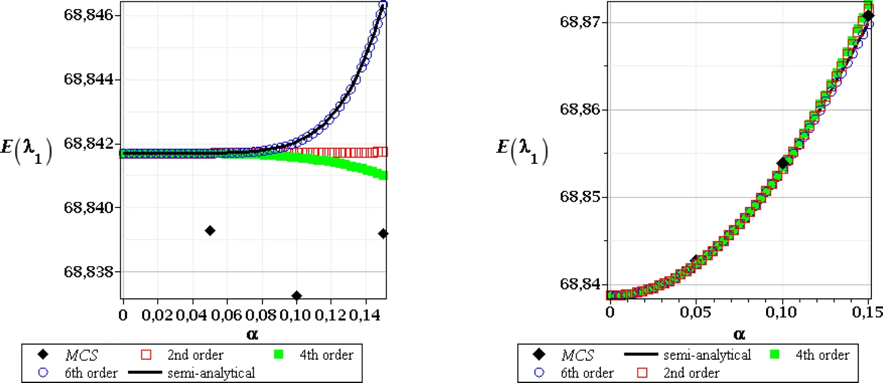
Figure 2:Expected values of the 1st critical value,FOT,random e(left),and random t(right)

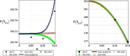
Figure 3:Expected values of the 13th critical value,FOT,random e(left),and random t(right)

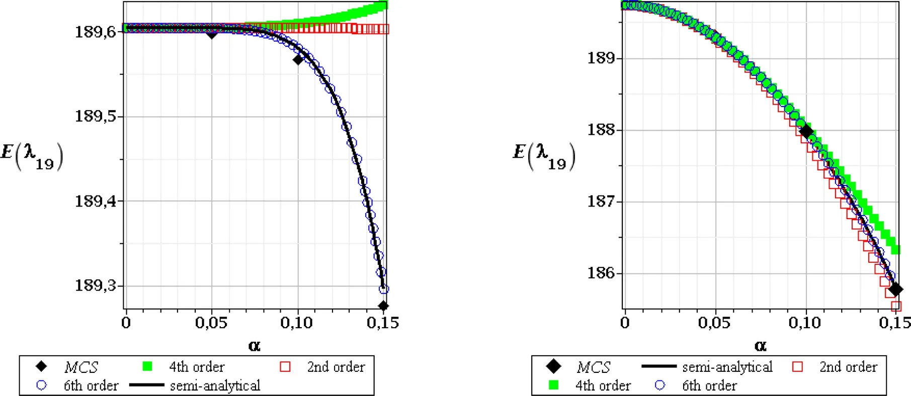
Figure 4:Expected values of the 19th critical value,FOT,random e(left),and random t(right)

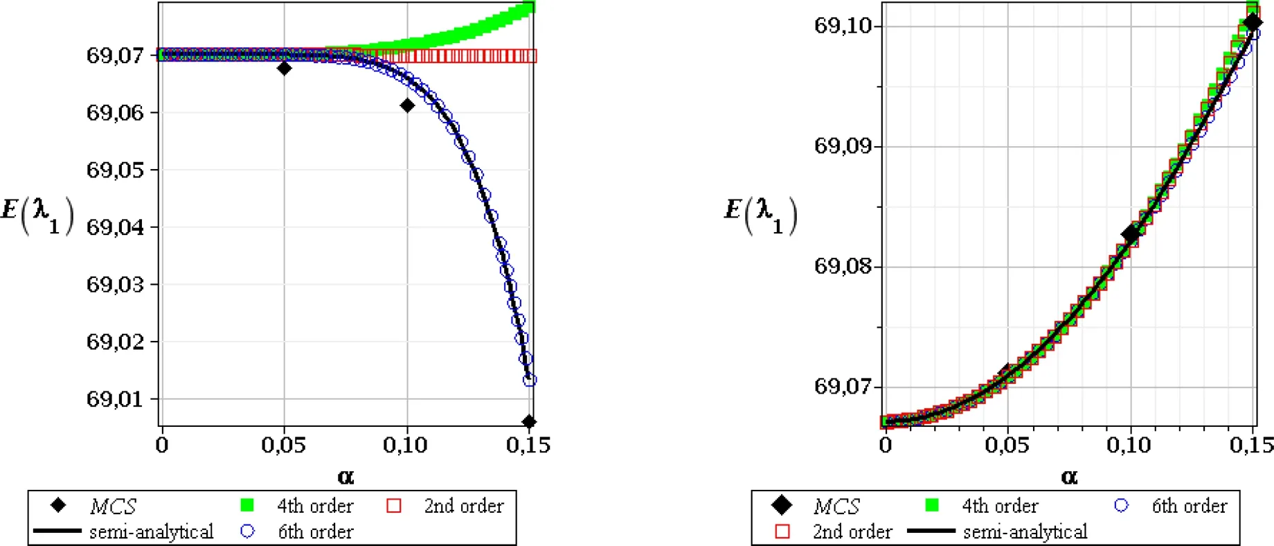
Figure 5:Expected values of the 1st critical value,SOT,random e(left),and random t(right)

Figure 6:Expected values of the 13th critical value,SOT,random e(left),and random t(right)

Figure 7:Expected values of the 19th critical value,SOT,random e(left),and random t(right)

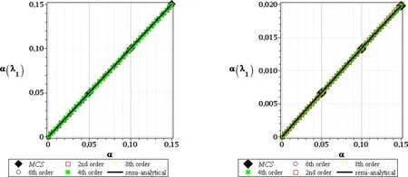
Figure 8:CoV of the 1st critical value,FOT,random e(left),and random t(right)

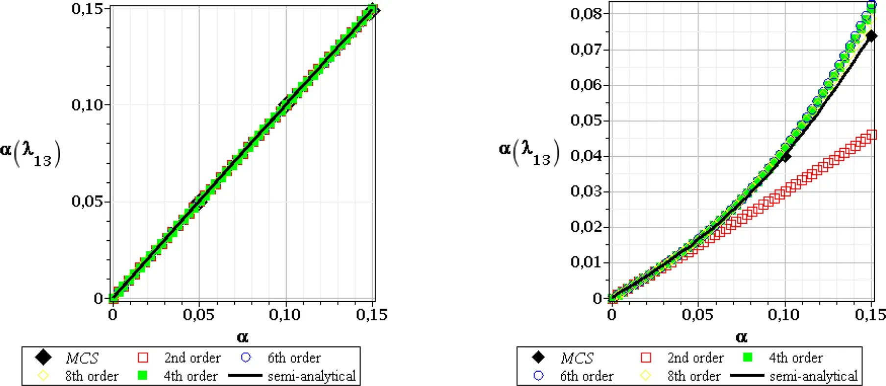
Figure 9:CoV of the 13th critical value,FOT,random e(left),and random t(right)

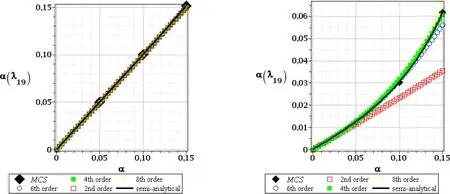
Figure10:CoVofthe19thcriticalvalue,FOT,randome(left),andrandomt(right)

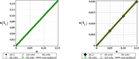
Figure 11:CoV of the 1st critical value,SOT,random e(left),and random t(right)

Figure12:CoVofthe13thcriticalvalue,SOT,randome(left),andrandomt(right)

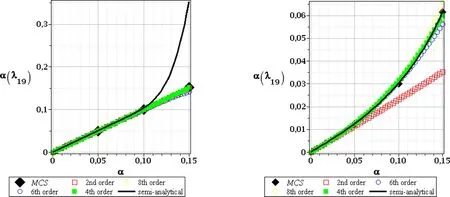
Figure13:CoVofthe19thcriticalvalue,SOT,randome(left),andrandomt(right)

The patterns and the values obtained for skewness of these three basic critical values are different for both input random variables.We apply consecutively the tenth order Taylor expansion after computational experiments included in[Kami´nski(2013)]and also because usually the weakest computational precision accompanies determination of the third central probabilistic moment and of the skewness.Randomization of Young modulus in the First Order Theory experiments gives the results very close to 0.They start to diverge forα(e)＞0.10 but this could be treated as a numerical discrepancy rather that is affected by the Least Squares Method itself rather than by an uncertainty in our computational analysis.Figs.14–16 document exactly that the 10thorder perturbation analysis,the semi-analytical approach and the Monte-Carlo simulation appear close to each other for the entire range of the considered input stochastic fluctuations.The Second Order Theory for randome(Figs.17–19,left column)bring somewhat different results,but very similar conclusions:the resulting skewness is either positive or negative as well,but the magnitude of absolute values ranges even with the few orders.Nevertheless,the initial range ofα(e)∈[0.00,0.10]returns the same result:the skewness is 0,so that the final PDF of the critical forces may be really treated as symmetric.It should be mentioned that its further divergence from 0 is not typical only for the stochastic perturbation method;even the Monte-Carlo simulation estimators are not equal 0 forα(e)＞0.10.The skewness resulting from uncertainty in the leg thickness differs from 0 for all the methods,for all the critical values and also for both stability theories.The only trivial exception is atα(t)=0 when obviously all the probabilistic approaches should theoretically return zeroes for the coefficient of variation,skewness and kurtosis at the same time because of determinism of such a problem.The second very apparent tendency here is the fact that the semi-analytical method gives exactly the same values as the Monte-Carlo simulation scheme;it remains true for the full range of the input uncertainty.It seems that the highest order stochastic perturbation technique is the closest to this principal trend,while the d-ifferences in-between the neighboring orders decreases for an increasing order of Taylor expansion itself.The next difference to randomeis an exact coincidence of the skewness obtained in the first and in the second order theory,where the 1stcritical value exhibits very small positive skewness,while the next two have apparently negative ones.We may also notice that the higher the critical value,the larger the absolute value of its skewness.Moreover,all the skewness curves contained in Figs.14–19 present continuous functions with no local oscillations that keep constant convexity everywhere;constant monotonicity is preserved for most of them as only the few of them have local extreme points.Kurtosis is the last probabilistic coefficient compared in this analysis and is presented in Figs.20–22 for the first order stability theory as well as in Figs.23–25–for the second order approach.The major tendencies observed in case of skewness remain valid in this case also.Randomization of Young modulus results in slightly different kurtosis for the first and for the second order theories for each critical value.Their extreme values obtained according to the first order method are smaller than these resulting from the SOT.Once more we need to postpone the results computed forα(e)＞0.10 as they seem to be too much affected by some additional numerical instabilities and where all the probabilistic numerical methods apparently diverge.The results obtained from the semi-analytical simulation and the highest order perturbation techniques are very close to each other but some minor differences are noticeable for a specific combination of the given critical force and of the input coefficient of variation.However,contrary to the previous probabilistic characteristics,kurtosis for random thickness shows different values in various probabilistic methods.It is rather distant from 0(with some exception in case of the first critical value),appears to be both positive and negative as well as systematically increases its absolute values together with an increasing coefficientα(t).The semi-analytical method and Monte-Carlo simulation schemes return here very similar results but their coincidence is a little bit weaker than in case of the skewness.

One may therefore conclude after verification of the coefficients of variation,skewness,and kurtosis that the PDFs of output critical forces could be treated as Gaussianwhile randomizing Young modulus of the steel. So that determination of higher order statistics is irrelevant as they could be treated as 0;this is not the case of random thickness for a group of several structural elements.Its Gaussian character includes the PDF of critical loading that varies significantly from the well-known bell shaped curve.It should be finally mentioned that the left series of the reliability indices theoretically better approximate the real durability of the tower,because PDF of the critical forces may be treated with better accuracy as a Gaussian one,unlike for randomt.

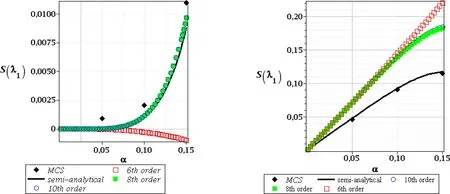
Figure 14:Skewness of the 1st critical value,FOT,random e(left),and random t(right)

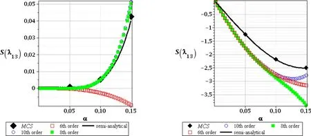
Figure 15:Skewness of the 13th critical value,FOT,random e(left),and random t(right)

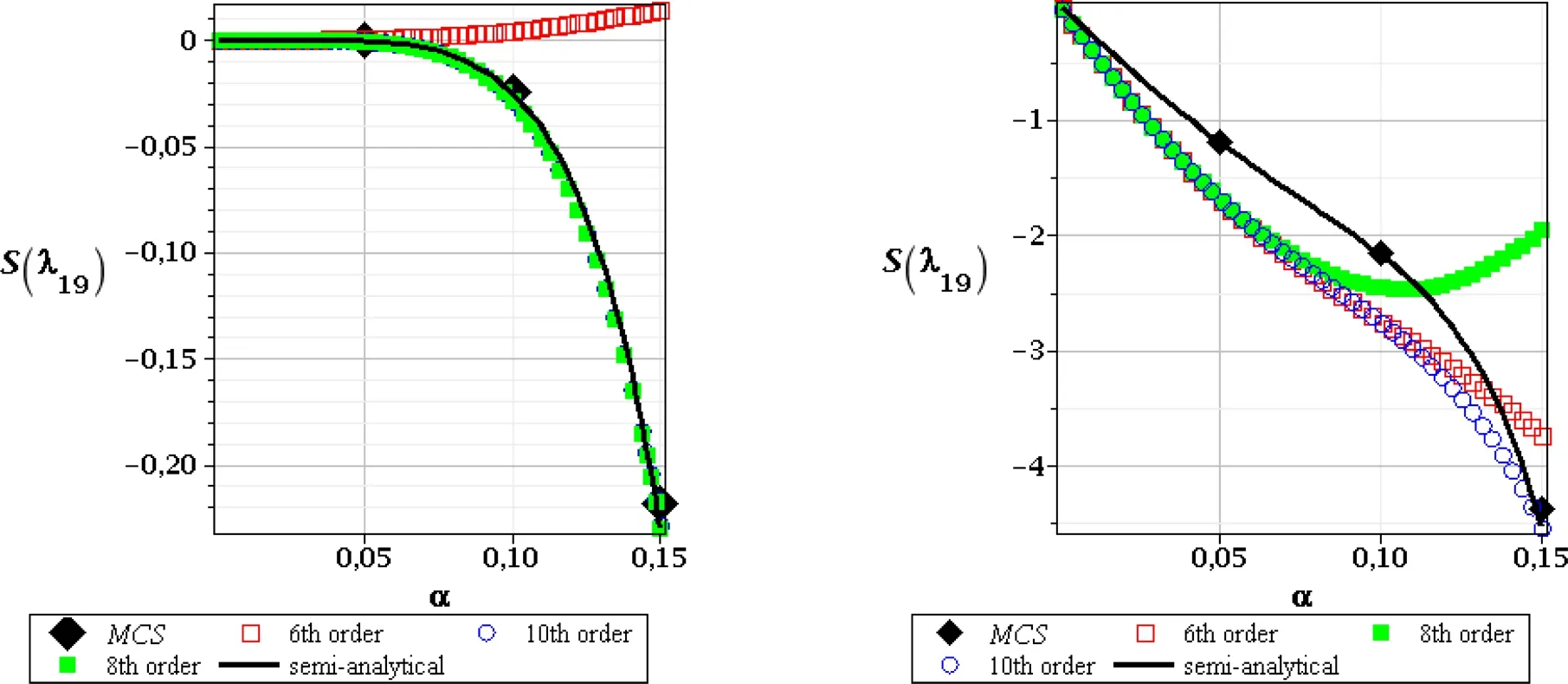
Figure 16:Skewness of the 19th critical value,FOT,random e(left),and random t(right)

Figure 17:Skewness of the 1st critical value,SOT,random e(left),and random t(right)

Figure 18:Skewness of the 13th critical value,SOT,random e(left),and random t(right)

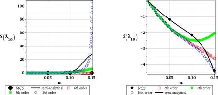
Figure 19:Skewness of the 19th critical value,SOT,random e(left),and random t(right)

Figure 20:Kurtosis of the 1st critical value,FOT,random e(left),and random t(right)

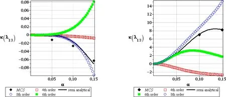
Figure 21:Kurtosis of the 13th critical value,FOT,random e(left),and random t(right)

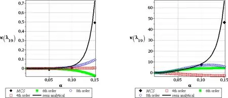
Figure 22:Kurtosis of the 19th critical value,FOT,random e(left),and random t(right)

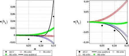
Figure 23:Kurtosis of the 1st critical value,SOT,random e(left),and random t(right)

Figure 24:Kurtosis of the 13th critical value,SOT,random e(left),and random t(right)

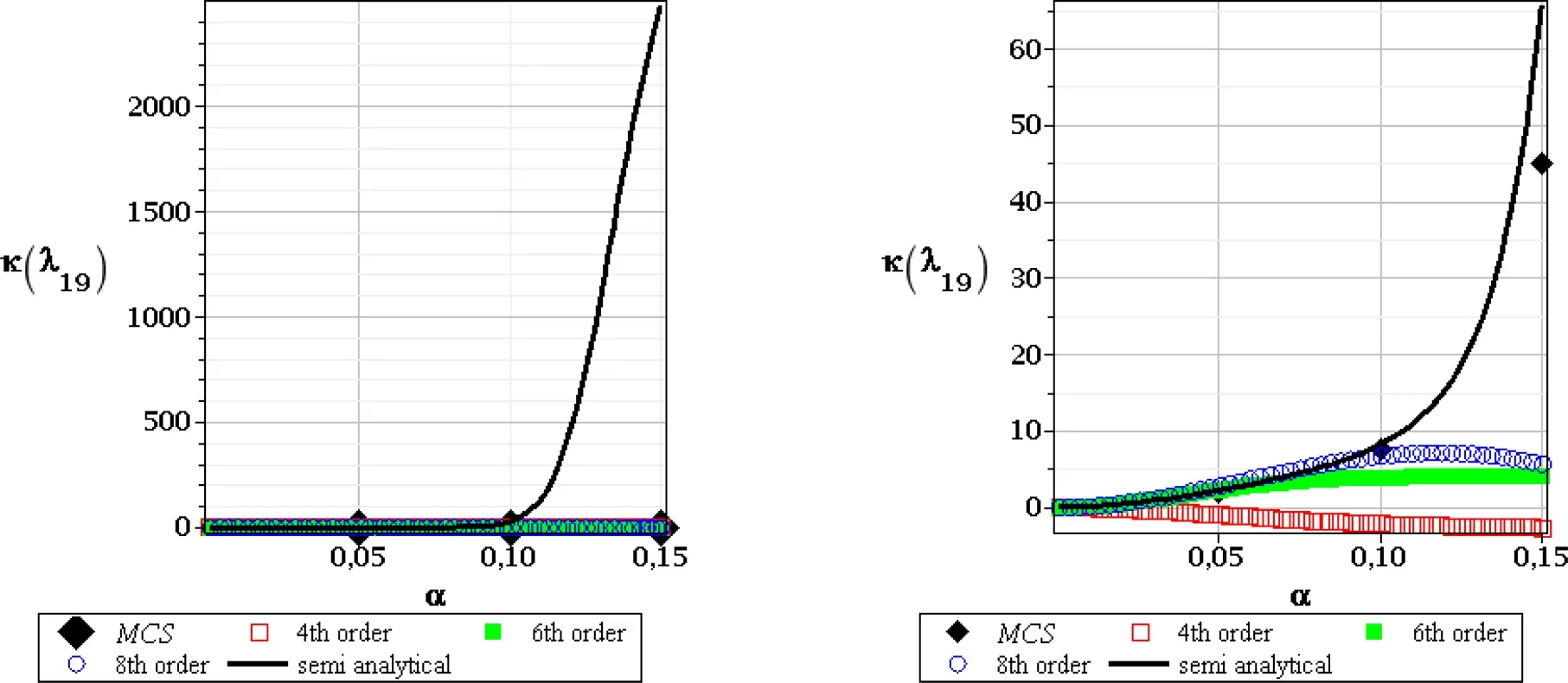
Figure 25:Kurtosis of the 19th critical value,SOT,random e(left),and random t(right)

Figure 26:Reliability index of the 1st critical value,FOT,random e(left),and random t(right)

Figure 27:Reliability index of the 13th critical value,FOT,random e(left),and random t(right)

Figure 29:Reliability index of the 1st critical value,SOT,random e(left),and random t(right)

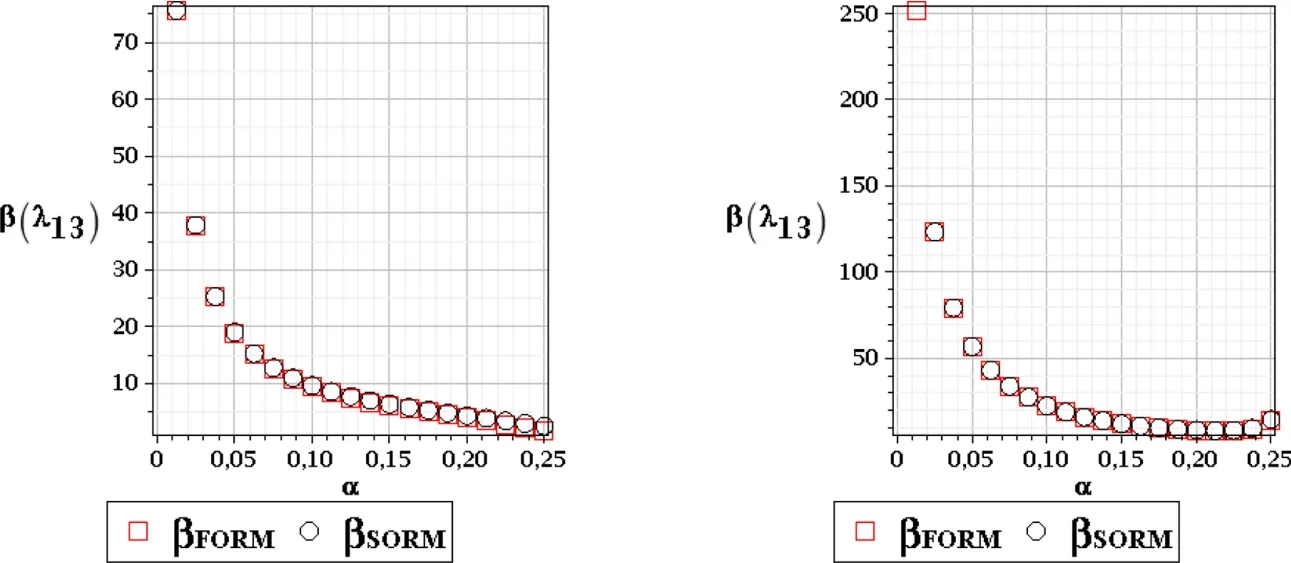
Figure 30:Reliability index of the 13th critical value,SOT,random e(left),and random t(right)

Figure 31:Reliability index of the 19th critical value,SOT,random e(left),and random t(right)

The reliability indices contained in Figs.26–28 for the First Order Theory and fur-ther in Figs.29–31 calculated according to the Second Order approach are drawn for a little bit wider range of input coefficientαthat belongs to the interval[0.00,0.25].This is done to use these results,especially right series,for further durability assessment in a presence of the corrosion process that usually increases significantly the uncertainty in structural element thickness.These indices are computed twice for both First and Second Order Reliability Methods,where we use the expectations and variances from the highest order stochastic perturbation method.Randomization of Young modulus and the thickness bring the same exponential shape of the reliability curves that naturally reaches maximum atα=0 and tends to 0 when increasing the input coefficientα.The results returned by the FORM and SORM are very close to each other(almost equal)throughout the full range of both input coefficients of variation;some differences may be noticed when one reduces the horizontal scale to[0.20,0.25],whereβSORMprevails.A contrasts of Figs.26 with 29,27 with 30 as well as 28 with 31 shows that the indices returned by the First and Second order theories are the same for the corresponding critical values,which follows the results obtained above for the first two moments.A comparison of the left series in Figs.26–31 enables to detect that the reliability curve remains the same for all studied critical values under Young modulus uncertainty.This is not the case of random thickness,where the first critical value is adjacent to the largest initial extreme value ofβ,then we have in turn 19thand 13thcritical values extremes,but generally the values obtained with randomtare larger than these adjacent to random Young modulus.This is mainly driven by the fact that we randomize elastic modulus uniformly in all structural elements of the tower,while element thickness is being randomized in the legs only;this apparently has local character.

5 Concluding remarks

1.Computational analysis provided in this paper shows that the weakest elements of a tower structure considering its additional stability,are the upper diagonal bracing members close to its top.The critical force adjacent to its stability loss is a few times smaller than that corresponding to buckling of the legs.It is due to the fact that they exhibit the largest ratio of a normal force(resulting from the technological loads increased during our numerical experiments)to their dead load.Gaussian uncertainty in Young modulus returns the critical forces that can be treated as Gaussian with a satisfactory accuracy,while randomization of leg thickness induces apparently non-Gaussian critical forces.The Gaussian character in case of the first random variable is concluded after the fact that the output CoV is equal to the input one,whereas skewness and kurtosis both are very close to 0(whenα(e)≤0.10,which gives a validity range for this conclusion).Generally,all three various proba-bilistic methods:semi-analytical,simulation and highest order stochastic perturbation technique returned very similar results,which additionally are almost equal in most cases for the entire variability range of the input coefficient of variation.The reliability indices computed with the use of FORM and SORM algorithms separately are almost exactly the same.They decrease exponentially with an increase of input uncertainty and they have smaller values for randomized Young modulus than for local random changes of the structural elements thickness.

2.One of next important issues in Stochastic Finite Element Method stability analysis of steel structures would be(1)an application of various order shell finite elements in order to model some local instability phenomena and(2)the additional finite element discretization of the welded and/or bolted connections[Hadianfard and Razani(2003);Papadopoulos,Stefanou and Papadrakakis(2009)].Such an extended analysis may include stochastic corrosion processes in steel elements subjected to the atmospheric environment,which usually has de finitely local character[Sadovský and Drdácký (2001)].The separate,very important issue would be post-buckling analysis of the steel towers where computational determination of the additional paths[Schafer and Graham-Brady(2006);Steinböck,Jia,Hö finger,Rubin and Mang(2008)],especially in the stochastic context(with the use of generalized stochastic perturbation technique)including reliability analysis using FORM and SORM,can be of the paramount importance;the analogous numerical issues concern the aluminum structures[Kami´nski,M.;Solecka,M.(2013)].

Björck,A.(1996):Numerical methods for least squares problems.SIAM,Philadelphia.

Elishakoff,I.(1983):Probabilistic Methods in the Theory of Structures.Wiley,New York.

Elishakoff,I.;Li,Y.W.;Starnes,J.H.(2001):Non-classical Problems in the Theory of Elastic Stability.Cambridge University Press,Cambridge.

Hadianfard,M.A.;Razani,R.(2003):Effects of semi-rigid behavior of connections in the reliability of steel frames.Struct.Safety,vol.25,pp.123–138.

Hosseini,S.M.;Shahabian,F.;Sladek,J.;Sladek,V.(2011):Stochastic meshless method for thermos-elastic wave propagation analysis in functionally graded thick hollow cylinders.CMES:Computer Modeling in Engineering and Sciences,vol.71,no.1,pp.39-66.

Huang,X.;Aliabadi,M.H.;Sharif Kodei,Z.(2014):Fatigue crack growth reliability analysis by stochastic Boundary Element Method.CMES:Computer Modeling in Engineering and Sciences,vol.102,no.4,pp.291-330.

Kami´nski,M.(2013):The Stochastic Perturbation Method for Computational Mechanics.Wiley,Chichester.

Kami´nski,M.;Solecka,M.(2013):Optimization of the aluminium and steel telecommunication towers using the generalized perturbation-based Stochastic Finite Element Method.Finite Elem.Analysis Design,vol.63(1),pp.69-79.

Kami´nski,M.;Str˛akowski,M.(2013):On the least squares stochastic finite element analysis of the steel skeletal towers exposed to the fire.Arch.Civ.&Mech.Engrg.,vol.13,pp.242-253.

Kami´nski,M.;Szafran,J.(2012):Stochastic finite element analysis and reliability of steel telecommunication towers.CMES:Computer Modeling in Engineering and Sciences,vol.83,no.2,pp.143-168.

Kleiber,M.(1985):Finite Element Method in Nonlinear Continuum Mechanics(in Polish).Polish Scientific Publishers,Warsaw-Pozna´n.

Kleiber,M.;Hien,T.D.(1992):The Stochastic Finite Element Method.Wiley,Chichester.

Kleiber,M.;Hien,T.D.(1997):Parameter sensitivity of inelastic buckling and post-buckling response.Comput.Meth.Appl.Mech.Engrg.,vol.145,pp.239-262.

Lin,S.;Liu,X.;Yuan,Y.;Mang,H.A.(2014):Constitutive modeling of earlyage concrete by a stochastic multi-scale method.CMES:Computer Modeling in Engineering and Sciences,vol.100,no.3,pp.157-200.

Melchers,R.E.(1987):Structural Reliability.Analysis and Prediction.Ellis Horwood Limited.

Papadopoulos,V.;Stefanou,G.;Papadrakakis,M.(2009):Buckling analysis of imperfect shells with stochastic non-Gaussian material and thickness properties.Int.J.Sol.&Struct.,vol.46,pp.2800-2808.

Sadovský,Z.;Drdácký,M.(2001):Buckling of plate strip subjected to localised corrosion—a stochastic model.J.Thin-Walled Struct.,vol.39,pp.247-259.

Schafer,B.W.;Graham-Brady,L.(2006):Stochastic post-buckling of frames using Koiter’s method.Int.J.Struct.Stability Dyn.,vol.6,pp.333-358.

Silva,C.R.A;Azikride Deus,H.P.;Mantovani,G.E.;Beck,A.T.(2010):Galerkin solution of stochastic beam bending on Winkler foundations.CMES:Computer Modeling in Engineering and Sciences,vol.67,no.2,pp.119-150.

Sokoł owski,D.;Kamin´ski,M.;Stra˛kowski,M.(2014):Stochastic Finite Element Method reliability analysis of the corrugated I-beam girder.CMES:Computer Modeling in Engineering and Sciences,vol.99,no.3,pp.209-231.

Steinböck,A.;Jia,X.;Hö finger,G.;Rubin,H.;Mang,H.A.(2008):Remarkable postbuckling paths analyzed by means of the consistently linearized eigenproblem.Int.J.Num.Meth.Engrg.,vol.76,pp.156-182.

Timoshenko,S.P.;Gere,J.M.(1961):Theory of Elastic Stability.McGraw-Hill,New York.

Wang,C.;Gao,W.;Yang,C.W.;Song,C.M.(2011):Non-deterministic structural response and reliability analysis using a hybrid perturbation-based stochastic finite element method and quasi Monte Carlo method.CMC:Computers,Materials and Continua,vol.25,no.1,pp.19-46.

Yang,Z.;Li,K.;Cai,Q.(2013): Universal reliability method for structural models with both random and fuzzy variables.CMES:Computer Modeling in Engineering and Sciences,vol.95,no.2,pp.143-171.

1This paper has been written on the occasion of the 70thanniversary of Łód´z University of Technology and the 60thanniversary of its Faculty of Civil Engineering,Architecture and Environmental Engineering.

2Head of Chair of Structural Reliability,Department of Structural Mechanics,Faculty of Civil Engineering,Architecture and Environmental Engineering,Al.Politechniki 6,90-924 Łód´z,Email:Marcin.Kaminski@p.lodz.pl

3Chair of Structural Reliability,Department of Structural Mechanics,Faculty of Civil Engineering,Architecture and Environmental Engineering,Al.Politechniki 6,90-924 Łód´z,Email:Jacek.Szafran@p.lodz.pl