A 3-D Visco-Hyperelastic Constitutive Model for Rubber with Damage for Finite Element Simulation

Ala Tabieiand Suraush Khambati

A 3-D Visco-Hyperelastic Constitutive Model for Rubber with Damage for Finite Element Simulation

Ala Tabiei1and Suraush Khambati2

A constitutive model to describe the behavior of rubber from low to high strain rates is presented.For loading,the primary hyperelastic behavior is characterized by the six parameter Ogden’s strain-energy potential of the third order.The rate-dependence is captured by the nonlinear second order BKZ model using another five parameters,having two relaxation times.For unloading,a single parameter model has been presented to define Hysteresis or continuous damage,while Ogden’s two term model has been used to capture Mullin’s effect or discontinuous damage.Lastly,the Feng-Hallquist failure surface dictates the ultimate failure for element deletion.The proposed model can accurately predict the response of rubber using a limited set of experimental data.The model has been validated here for the case of rubber but can be extended to a wide range of polymers.

hyperelasticity,viscoelasticity,hysteresis,Mullin’s effect,rubber,constitutive.

Nomenclature

λ1,λ2,λ3Principal Stretches

W Strain-energy potential

µ1,µ2,µ3Material Constants(Shear moduli)for Ogden’s Strain-energy potential

α1,α2,α3Material Constants(Exponents)for Ogden’s Strain-energy potential

G Shear Modulus

σ Cauchy’s stress tensor

F Deformation gradient

dx Infinitesimal material element in deformed configuration

dX Infinitesimal material element in reference configuration

J Jacobian

C Right Cauchy-Green deformation tensor

˙C Rate of Change of Right Cauchy-Green deformation tensor

˙F Rate of Change of Deformation gradient

P 1stPiola-Kirchhoff stress

S 2ndPiola-Kirchhoff stress

p Hydrostatic pressure

c Constant for pure homogenous deformation

σhHyperelastic component of Cauchy’s stress tensor

σvViscoelastic component of Cauchy’s stress tensor

pvPressure in viscoelastic material

Ω Matrix function

t Time

τ Time integral

ϕ Function of invariants of Right Cauchy-Green deformation tensor

I1,I2,I3Invariants of Right Cauchy-Green deformation tensor

M Relaxation function

˙E Strain rate

θ1,θ2Relaxation times

˙λStrain rate

C1,C2,C3Viscoelastic constants(in function of invariants)

C4,C5Viscoelastic constants(relaxation times)

S Stretch Integral

φ (η) Function of Damage

η Damage variable

α Damage parameter

λmMaximum stretch at which unloading starts

PuUnloading value of 1stPiola-Kirchhoff stress

WOPrimary Strain-energy potential

r,m Material constants for Mullins’effect

erf Error function

WmStrain-energy potential at maximum stretch

ηmMinimum value of damage variable(at complete unloading)

Ψ Failure criteria

β Constant for Feng-Hallquist failure surface

1 Introduction

Rubber is commonly used in automotives as tires,transmission belts,hoses,gaskets,seals,vibration isolation mounts,interlayer in windshields,and in architectural applications as transparent armor and ballistic protection.Thus,depending on the intensity and frequency of the load,rubber exhibits deformation over a range of strain-rates varying from low to high.Due to their hyperelastic nature,rubberlike polymers can withstand large strains without undergoing permanent deformation,hence providing large energy absorption.Therefore,it is necessary to have a constitutive model that can incorporate its’various characteristics including ratesensitivity,creep, relaxation,hysteresis and Mullin’s effect.

Here,a phenomenological stretched-based constitutive model has been developed for rubber, which is consistent within the laws of continuum mechanics and theories of deformation.The mathematical formulation of new and existing models has been presented toward developing one unified model.The various sections which this study focuses on,can be summarized as follows:

1.Hyperelasticity – Ogden’s hyperelastic strain energy potential of the third order was used to characterize the primary material response,i.e.hyperelasticity[Ogden(1972)].

2.Viscoelasticity – the viscoelastic component of the Cauchy’s stress is given by the BKZ model[Zapas(1966)]of order two–implying two relaxation times–each corresponding to low strain rates of 10−4mm/mm/s to 10−1mm/mm/s and high strain rates of 102mm/mm/s to 103mm/mm/s.

3.Hysteresis–intended for modeling large-strain rate-dependent behavior of elastomers.Here the corresponding primary foam behavior is scaled by the damage variable to provide the unloading response.It is a continuous type of damage.

4.Mullins’effect– is used for modeling the stress softening of filled elastomers(like rubber)under quasi-static loading.The material requires less stress on reloading than initial loading for stretches up to maximum stretch during initial loading. This stress softening behavior is called as Mullins effect and it reflects the damage incurred during previous loading cycles[Mullins(1969)].The energy required to cause damage is not recoverable.Damage occurs at microscopic level by severing bonds between filler particles and rubber molecular chains.It is a discontinuous type of damage.

5.Failure Surface–The Feng-Hallquist failure surface has been studied and

suggested as a suitable model wherein data from stretch-to-failure experi-mental tests is required to completely characterize the model and obtain material parameters[Feng(2007)].

In what follows,each of the above mentioned topics is presented and discussed in detail.

2 Constitutive Model

2.1 Hyperelasticity

A hyperelastic material is a type of constitutive model for ideal elastic materials for which the stress-strain relationship is derived from a strain-energy density function.In this particular section,we assume the hyperelastic response as non-linear elastic,isotropic,incompressible and independent of strain-rate.

Ogden developed a sophisticated way for simulating incompressible(rubber-like)materials like biological soft tissues and solid polymers which undergo finite strains relative to an equilibrium state in the phenomenological context[Ogden(1972)].The postulated strain energy is a function of the principal stretches λa,a=1,2,3.The Ogden hyperelastic strain energy potential is given by

The conventional Shear Modulus G(in the undeformed,stress-free or natural configuration)is given by

For incompressible materials,

Now,in order to obtain stress in terms of the strain-energy potential,let’s state a few important relationships.Internal forces are represented by Cauchy’s stress tensor σ and F is the deformation gradient.The deformation gradient F is given by[Holzapfel(2000)and Hutter(1993)]:

with the Jacobian,J=det(F),which is the ratio of volumes in current and deformed configurations.

The right Cauchy-Green deformation tensor is defined in terms of F as

The rate of change of the right Cauchy-Green deformation tensor is given as[Hutter(1993)and Bower(2009)]

In terms of the 1stPiola-Kirchhoff stress:

In terms of the 2ndPiola-Kirchhoff stress:

Now,we can write the Cauchy’s stress in terms of the strain-energy potential as

where p is the hydrostatic pressure.

The first Piola-Kirchoff Stress(1stPK)is

The following cases of principal stretch values λa,a=1,2,3,in terms of stretch in the primary direction λ,are particularly useful while using experimental data:

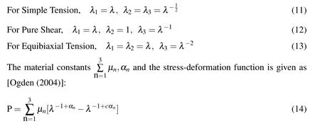
where P=Force per unit undeformed area or 1stPK stress,

c=Pure homogeneous deformation.

For simple tension c=−1/2,

For pure shear c=−1,and,

For equi-biaxial tension c=−2.

2.2 Viscoelasticity

A real system exhibits behavior which is a combination of solid and liquid like characteristics.Some of the energy input is stored and recovered in each cycle while some is dissipated as heat.Such materials are called viscoelastic.If both strain and stress are infinitesimal,then the body exhibits linear viscoelasticity[Ferry(1961)].The overall response of the material can thus be written as:σ=σh+σv.

The viscoelastic component as given by the BKZ Model[Bernstein(1963),Bernstein(1965)and Yang(2004)]is:

where pvis the pressure in the viscoelastic material.

The matrix function is:

The strain rate is given by the following equation:

And the relaxation function is:

where θiis the relaxation time.We consider N=2,following the BKZ model:

θ1corresponds to low strain rates of 10−4to 10−1mm/mm/s

θ2corresponds to high strain rates of 102to 103mm/mm/s

Once we obtain the hyperelastic constants,we can find the viscoelastic constants next.Here,taking the strain rate 0.01 mm/mm/s assuming it to be quasi-static,we use the six hyperelastic constants to characterize the quasi-static response.For the case of uniaxial extension,we have the deformation gradient as[Yang(2004)and Yang(2000)]:

Also,the invariants of the right Cauchy-Green deformation tensor are given by:

In equation(16)and(18),t−τ is the amount of time that has elapsed between τ and t,so we consider contributions from all τ＜ t[Silva(2008)].Thus,effect of deformation history on stress for τ＜ 0 at time t＞ 0 is ignored.

Redefining the integration limits in terms of stretch:

In equation(15)for σv,we assume the following form for φ ,

Since the relaxation times θ1and θ2are constants,they will be referred to as C4and C5respectively.Thus,we can write the viscoelastic component of stress at time t,by substituting(16)(17)(18)and(23)in equation(15),as

Where the strain-rate from(17)and(19)is

Since t is a constant for integration and τ is a time variable,we can rewrite(21)in terms of its’principal components as

Substituting the value for pvin the above equations in(26),we get equation(27)as follows,which we curve fit to experimental data:

While τ ranges from(0,t),the stretch integral S ranges from(1,λ ),thus we can write:

where t corresponds to final stretch λ ,while τ corresponds to current stretch S.Thus,in the curve fitting equation(27)forwe substitute all values of λ by S in the curly parentheses{},because it is a variable to be integrated between(0,t)or(1,λ).

Since in our case we have data at three different strain rates,we can determine theor the viscoelastic stress components for the three test curves.Thus,for each of the curves,we can get the hyperelastic component of stress by subtracting each viscoelastic stress component from the test curve asThe three new curvesshould almost superimpose into a single curve,in order to validate the correctness of the model.

2.3 Hysteresis

Filled elastomers exhibit dissipative properties leading to hysteresis in cyclic loadstrain curves due to chain-breakage,micro-structural damage and micro-void formation.In other words,since some energy is lost or dissipated as heat,they require more energy during loading than upon unloading.A stretch-based framework is proposed for modeling the continuum damage behavior of rubber and to simulate fatigue behavior.

Hysteresis is intended for modeling large-strain rate-dependent behavior of elastomers.Energy dissipation through hysteresis is represented by the area between the loading and unloading curves in a load-deformation cycle,and occurs in all types of rubber.The complementary property of hysteresis is resilience,which is a measure of the energy returned during each cycle.

The augmented energy potential is given[Dorfmann(2003)]as:

where W(λ)is the strain-energy potential during loading and η is the damage variable.

Atη =0,no damage occurs and W(λ,0)=W(λ)or the primary curve is followed.The Cauchy’s stress is given by

where σ (λ)corresponds to primary foam behavior,scaled by the damage variable(1−η).

Next,to define the damage variable η[Calvo(2009)],we employ a stretch-based form as given below:

where λmis the maximum value of λ during the deformation history and α is a dimensionless material parameter.

The energy dissipated due to damage in the material is given by φ (ηm),and the recoverable part of energy is given by:

Now,for computing the damage parameter α for unloading during an experiment,say uniaxial hyperelastic extension,we first find the hyperelastic constants as described earlier.Next we separate the data into the tensile and compressive zones for the unloading curve.Now, starting off with the tensile curve, we find the maximum stretch on the loading curve,call it max.Then for every data point on the unloading curve,say,current stretch we compute the 1stPK stress as:

As in(30),we compute the unloading stress value by scaling it by(1−η)as follows:

2.4 Mullins’effect

Mullins effect is used for modeling the stress softening of filled rubber-like elastomers under quasi-static loading[Mullins(1969)and Dorfmann(2003)].Elastomers soften significantly when exercised and this strain softening is most pronounced between the first and second cycles,then usually disappearing between the third and fourth cycles.Thus,Mullins’effect is a discontinuous type of damage evolution.

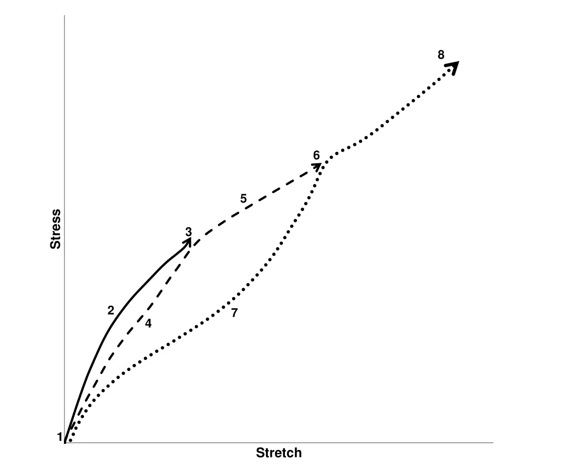
Figure 1:Mullins’effect schematic representation.

Figure 1 represents Mullins’effect schematically.In the figure one can observe the following:

1.Curve 1-2-3 is the primary loading path

2.Curve 3-4-1 is the unloading path from point 3

3.Curve 1-4-3 is the reloading path up to point 3

4.Curve 3-5-6 is the reloading path beyond point 3

5.Curve 6-7-1 is the unloading path from point 6

The augmented energy potential is given by the following equation:

where η is the damage variable and φ (η)is a function of damage.

The Cauchy’s stress is given by:

where σ (λ)corresponds to primary foam behavior,scaled by the damage variable η.

Let λmbe the point where unloading has most recently initiated,the unloading stress at a particular stretch is given by multiplying the stress at loading by the damage variable η.Upon reloading,if λ ＞＞ λmthen η =1,or in other words the primary load path is active after stretching beyond the maximum stretch attained in the previous loading cycles.

We assume the following form of the damage variable as proposed by Ogden-Roxburgh[Ogden(1988)]:

where r,m are positive parameters or material constants,and erf is the error function which is suitable to capture the nature of the unloading curve and is given by the following:

At λ1= λ2=1,when the material is fully unloaded,η attains it’s minimum value ηmand φ (ηm)is the residual(or non-recoverable energy)which gives the measure of the energy required to cause damage in the material.In a uniaxial experiment,φ (ηm)equals to the area between primary loading curve and relevant unloading curve.

The recoverable part of the energy is given by:

At the microscopic level,stress softening is associated with the damage caused by loading by severing the bonds between the filler particles and the rubber molecular chains.

The total damage is thus given by[Miehe(1995)]:

2.5 Failure surface

In most structural applications,the finite element method is used to predict failure.This is done by comparing the calculated solution to some failure criteria.The failure description for rubber used here is the general failure criterion for polymers as given by Feng and Hallquist[Feng(2005)and Feng(2007)].The failure surface is based on the energy principle–when the strain energy reaches a maximum,the material fails.Although,rubber may fail when subjected to repeated applied stress cycles even when they are well below the single cycle breaking stress.

In terms of the deformation gradient F,the failure surface is given by the following:

For incompressible materials,I3=1 and the failure surface in(38)simplifies to

Further expanding(42),we get the failure criterion for hyperelastic solids as

Any strain rate satisfying Ψ＜0 is below the failure state and represents a stress free state,thus β＜0 is required.Thus,failure surface is described by state in which β=0

where Γ1,Γ2and K are the 3 material failure constants and can be obtained from test data(a minimum of three tests are required).

3 Results and Discussion

3.1 Hyperelasticity

Ogden’s three-term model

For our validation,we first find the parameters for the three-term Ogden model in the following modes of deformation simultaneously:in simple tension,pure shear and equibiaxial tension.The data[Ogden(2004)]we use is given in Figure 2.Using the first set of values to iteratively converge at a solution such that the value of the sum of squares remains nearly constant so as to represent a stable set of values:as seen in Table 1. The curve fit is given by Figure 2 which captures all three modes of deformation very accurately with the same set of material parameters,as given by Table 2[Twizell(1983)].The order of stiffness is given by

Table 1:Minimizing function.

Table 2:Material parameters obtained for Ogden model.

3.2 Viscoelasticity

Quasi-static Response

Figure 2:Experimental data[19]for 8%S rubber in uniaxial tension,pure shear and equibiaxial tension fitted to the three-term Ogden model.

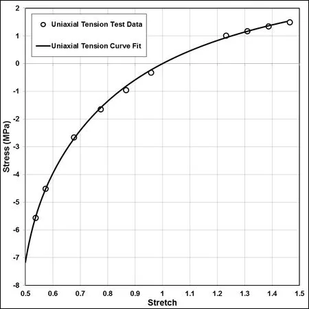
Figure 3:Experimental data[6]plotted against the proposed model for the quasistatic response of rubber at a strain-rate of 0.01 mm/mm/s.

In the previous section,we see that the hyperelastic model can capture deformation in various different modes.Next,we go on to evaluate the viscoelastic model for uniaxial case.In order to do this,we first need to obtain the hyperelastic parameters for the case of quasistatic loading as seen in Figure 3.The parameters are given in Table 3,which we use to obtain the viscoelastic parameters in the next section[Bois(2003),Benson(2006)and Bois(2006)].

Table 3:Hyperelastic constants.

Table 4:Viscoelastic constants.

Figure 4:Experimental data[6]plotted against the proposed model for the dynamic response of rubber at a strain-rate of 0.01,1.0 and 100.0 mm/mm/s.

Dynamic Response

After obtaining the hyperelastic parameters for the three-terms Ogden model,we find the parameters for the non-linear BKZ model while curve fitting our equation to both strain rates simultaneously,as given in Figure 4.The viscoelastic parameters,including the two different relaxation times,are given in Table 4.

3.3 Hysteresis

Quasi-static Response

Using the same set of data for the case of loading,as given by Figure 3,we find the unloading parameter for the case of hysteresis,for the tension and compression regions simultaneously.The experimental data and the model validation can be seen in Figure 5.The hysteresis material constant is given in Table 5 and is given in relation to the damage variable η as:

Table 5:Hysteresis constant.

Table 6:Hyperelastic constants for primary loading.

3.4 Mullins’effect

Primary Loading Response

Now for the case of Mullins effect,we consider another set of data,as shown in Figure 6.First,we have to characterize the primary hyperelastic response,thus obtaining the hyperelastic parameters as given in Table 6.

Figure 5:Experimental data[6]plotted against the proposed model for the unloading response of rubber using damage function at a strain-rate of 0.01 mm/mm/s.

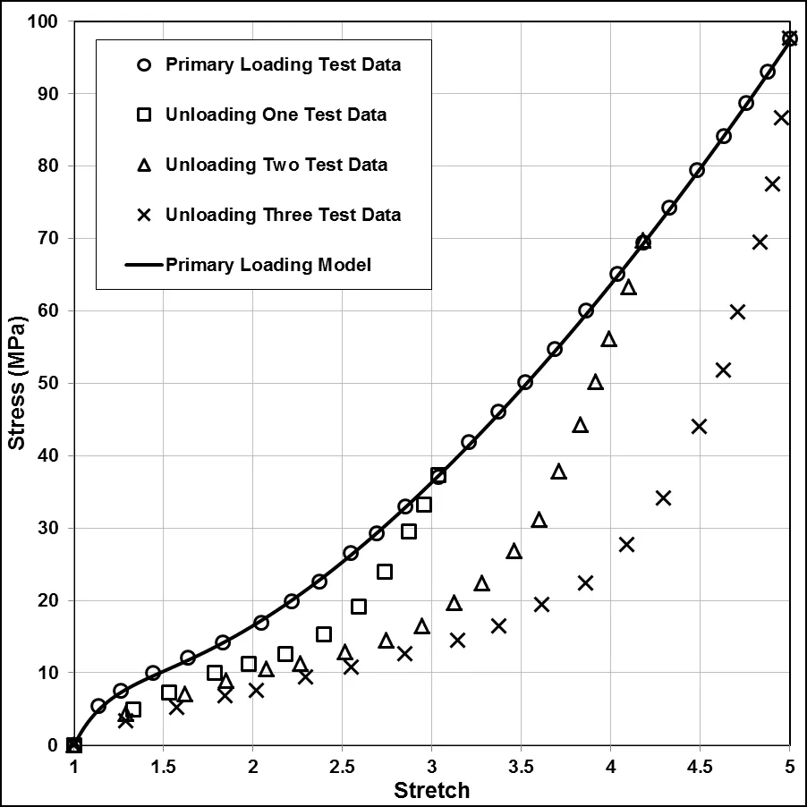
Figure 6: Experimental loading data [17] plotted against the hyperelastic three-term Ogden model for primary response of rubber compound.

Figure 7:Experimental unloading data[17]plotted against the proposed model for Mullins’effect up to second maximum stretch.

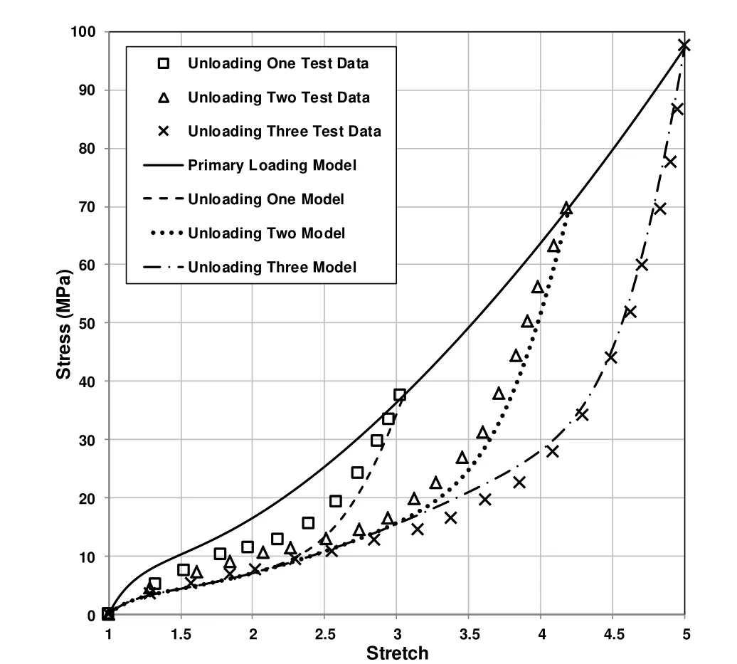
Figure 8:Experimental unloading data[17]plotted against the proposed model for Mullins’effect with third maximum stretch.

Unloading Response

Next,for unloading due to Mullins’effect,we have to find the parameters r and m,using data from all the points where unloading begins.We regard the first two points as our maximum stretch.The experimental data and the model can be seen in Figure 7.The parameters for the Mullins’effect are given in Table 7.We see that for the case of unloading using two points,we get a good fit but the model can also capture unloading from three points reasonably well.Therefore,for unloading including three maximum stretches,we again find the parameters r and m,using data from all three points where unloading begins.We regard these three points as our maximum stretch.The experimental data against the model can be seen in Figure 8.The parameters for the Mullins’effect now are given in Table 8.

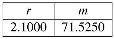
Table 7:Mullins effect constants for unloading with second maximum stretch.

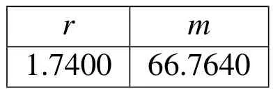
Table 8:Mullins effect constants for unloading with third maximum stretch.

4 Conclusion

A constitutive model is proposed to predict the response of rubber which is characterized by its’hyperelasticity,viscoelasticity, hysteresis and Mullins’effect.Based on experimental data,material parameters have been found and the constitutive models have been validated in a limited set of deformation modes.As seen in the results,one unified model can be used to capture the dynamic response of rubberlike polymers under different loading conditions with great accuracy.Since material is an intensive property,a constitutive model with a given set of parameters can be extended to a wide range of industrial applications.

Benson,D.J.;Du Bois,P.A.;Kolling,S.(2006):A simplified approach for strain-rate dependent hyperelastic materials with damage.9th International LSDYNA Users’Conference.

Bernstein,B.;Kearsley,E.A.;Zapas,L.J.(1963):A study of stress relaxation with finite strain.Transactions of the Society of Rheology,vol.VII,pp.391-410.

Bernstein,B.;Kearsley,E.A.;Zapas,L.J.(1965):Elastic stress-strain relations in perfect elastic fluids.Transactions of the Society of Rheology,pp.27-39.

Bower,A.F.(2009):Applied Mechanics of Solids.CRC Press.

Calvo,B.;Pena,E.(2009):On modelling damage process in vaginal tissue.Journal of Biomechanics,vol.42,pp.642-651.

Dorfmann,A.;Ogden,R.W.(2003):A pseudo-elastic model for loading,partial unloading and reloading of particle-reinforced rubber.International Journal of Solids and Structures,vol.40,pp.2699-2714.

Du Bois,P.A.(2003):A simplified approach to the simulation of rubber-like materials under dynamic loading.4th European LS-DYNA Users’Conference.

Du Bois,P.A.;Kolling,S.(2006):Material behaviour of polymers under impact loading.International Journal of Impact Engineering,vol.32,pp.725-740.

Feng,W.W.;Hallquist,J.O.(2005):A failure criterion for polymers and soft biological materials.5th European LS-DYNA Users’Conference.

Feng,W.W.;Hallquist,J.O.(2007):Numerical modelling and biaxial tests for the Mullins’effect in rubber.6th European LS-DYNA Users’Conference.

Ferry,J.D.(1961):Viscoelastic Properties of Polymers.Wiley Publications.

Holzapfel,G.A.(2000):Nonlinear Solid Mechanics:A Continuum Approach for Engineering.Wiley Publications.

Hutter,K.(1993):Continuum Mechanics in Environmental Science and Geography.Springer Publications.

Miehe,C.(1995):Discontinuous and continuous damage evolution in Ogden-type large-strain elastic materials.Eur.J.Mech.,A/Solids,vol.14,no.5,pp.697-720.

Mullins,L.(1969):Softening of rubber by deformation.Rubber Chemistry and Technology,vol.42,no.1,pp.339-362.

Ogden,R.W.(1972):Large deformation isotropic elasticity-on the correlation of theory and experiment for incompressible rubberlike solids.Proc.R.Soc.London A.,vol.326,no.1567,pp.565-584.

Ogden,R.W.;Roxburgh;D.G.(1999):A pseudo-elastic model for the Mullins effect in filled rubber.Proc.R.Soc.London A.,vol.455,no.1988,pp.2861-2877.

Ogden,R.W.;Saccomandi G.;Sgura,I.(2004):Fitting hyperelastic models to experimental data.Computational Mechanics.

Silva,H.N.;Soares,J.B.;Parente Jr.,E.;Sousa1,P.C.(2008):Implementation of a Viscoelastic Constitutive Model Using the Object-Oriented Programming Approach.Tech Science Press ICCES,vol.7,no.4,pp.181-188.

Twizell,E.H.;Ogden,R.W.(1983):Non-linear optimization of the material constants in Ogden’s stress-deformation function for incompressible isotropic elastic materials.J.Austral.Math.Soc.,ser.B 24,pp.424-434.

Yang,L.M.;Shim,V.P.W.;Lim,C.T.;Law,P.H.(2004):A visco-hyperelastic constitutive model to characterize both tensile and compressive behavior of rubber.Journal of Applied Polymer Science,vol.92,pp.523–531.

Yang,L.M.;Shim,V.P.W.;Lim,C.T.(2000):A visco-hyperelastic approach to modelling the constitutive behavior of rubber.International journal of impact engineering,vol.24,pp.545-560.

Zapas,L.J.(1966):Viscoelastic behavior under large deformations.Journal of Research of the National Bureau of Standards,vol.70A.

1Associate Professor.School of Advance Structures,College of Engineering and Applied Sciences,University of Cincinnati,OH 45221-0071,USA.E-mail:ala.tabiei@uc.edu

2Graduate Student.School of Advance Structures,College of Engineering and Applied Sciences,University of Cincinnati,OH 45221-0071,USA.E-mail:khambasq@mail.uc.edu