A method used to determine the upper thermal boundary of subgrade based on boundary layer theory

QingBo Bai， Xu Li，2*， YaHu Tian，2

1. School of Civil Engineering， Beijing Jiaotong University， Beijing 100044， China

2. Qinghai Research and Observation Base， Key Laboratory of Highway Construction & Maintenance Technology in Permafrost Regions， Ministry of Transport， Xining， Qinghai 810001， China

A method used to determine the upper thermal boundary of subgrade based on boundary layer theory

QingBo Bai1， Xu Li1，2*， YaHu Tian1，2

1. School of Civil Engineering， Beijing Jiaotong University， Beijing 100044， China

2. Qinghai Research and Observation Base， Key Laboratory of Highway Construction & Maintenance Technology in Permafrost Regions， Ministry of Transport， Xining， Qinghai 810001， China

In the numerical simulation of long-term subgrade temperature fields， the daily variation of soil temperature at a certain depth h is negligible. Such phenomenon is called the "boundary layer theory." Depth h is defined as the boundary layer thickness and the soil temperature at h is approximately equal to a temperature increment plus the average atmosphere temperature. In the past， the boundary layer thickness and temperature increment were usually extracted from monitored data in the field. In this paper， a method is proposed to determinate the boundary layer thickness and temperature increment. Based on the typical designs of highway or railway， the theoretical solution of boundary layer thickness is inferred and listed. Further， the empirical equation and design chart for determining the temperature increment are given in which the following factors are addressed， including solar radiation， equivalent thermal diffusivity and convective heat-transfer coefficient. Using these equations or design charts， the boundary layer thickness and temperature increment can be easily determined and used in the simulation of long-term subgrade temperature fields. Finally， an example is conducted and used to verify the method. The result shows that the proposed method for determining the upper thermal boundary of subgrade is accurate and practical.

temperature field； boundary layer； permafrost； subgrade； equivalent thermal diffusivity

1　Introduction

The simulation of subgrade temperature field is the foundation of the thermal stability analysis of subgrade in permanent and seasonal permafrost regions. In the numerical simulation of long-term subgrade temperature fields， it is difficult to accurately simulate the daily fluctuations of solar radiation and atmosphere temperature. By long-term observation，Zhu （1988） put forward the "boundary layer theory" as the upper thermal boundary to calculate the subgrade temperature field. The boundary layer theory assumes that the effect of daily solar radiation and air temperature are negligible at the bottom of the boundary layer； thus， soil temperature at the bottom of the boundary layer is equal to the atmosphere temperature plus a temperature increment.

Based on the boundary layer theory， boundary layer thickness and temperature increment are two major parameters involved in the upper boundary of subgrade in the numerical simulation of long-term temperature fields. Based on theoretical derivation，Bai et al. （2015） set up the theoretical solution of the boundary layer thickness and summarized the factors affecting the temperature increment.

Based on the typical designs of highway or railway，this paper sketches the design formulae of boundary layer thickness and the empirical equation of temperature increment. First， the subgrade pavement structures of typical roads are summarized， such as highway and railroad. Second， the boundary layer thicknesses are calculated and listed. Third， the main factors impacting the temperature increment are collected. Lastly， a numerical simulation is performed for the temperature field of a Qinghai-Tibet Highway embankment. The results are further compared with monitored data in the field.

2　The boundary layer theory of thermal conduction problem in pavement

2.1The boundary layer theory of thermal conduction problem

The boundary layer theory was first introduced in hydromechanics and used to describe that laminar flow will be present when water has a critical distance d from the boundary. A similar phenomenon is observed in the thermal conduction problem of subgrade where the daily variation of temperature at a certain depth beneath ground surface is negligible. Such phenomenon is first termed as the "boundary layer theory" by Zhu （1988）. Soil strata can be divided into three layers from top to bottom： convection heat exchange， radiation heat transfer， and heat-conduction； the radiation heat transfer layer is called "the boundary layer" （Zhu， 1988）. Yan （1984）indicated that the boundary layer thickness is soil depth without the daily effect of solar radiation and air temperature.

The soil temperature at the bottom of the boundary layer （δu） could be described by the equation：

where Tais the mean temperature which could be expressed with a periodic function in a year； Tiis the temperature increment； εdis the daily amplitude of the soil temperature； ωdis the angular frequency， equal to 2π/24h； φ is the epoch.

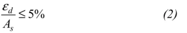
At a certain depth （δu）， εdis ignored as a small amount， meaning that the soil temperature is irrespective to the daily effect of solar radiation and air temperature. Therefore， the soil temperature at a certain depth （δu） could be regarded as the upper thermal boundary in the numerical simulation of a long-term subgrade temperature field， and the value of εdis set to zero to simplify the upper thermal boundary. The phenomena of boundary layer in subgrade could be described in Figure 1； the daily temperature amplitude in deeper soil is smaller， and the soil temperature is higher than air temperature.

Based on the boundary layer theory， boundary layer thickness （δu） and temperature increment （Ti） are two major parameters in determining the upper thermal boundary.

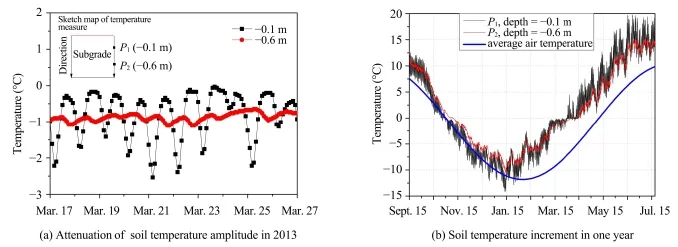
Figure 1　Temperature of monitoring points

2.2Conversion parameters in the boundary layer theory

In this paper， the criteria selecting boundary layer thickness is expressed with the equation：

where Asis the temperature amplitude of road surface.

The temperature amplitude in soil is smaller when the soil depth is larger. Bai et al. （2015） put forward the attenuation of temperature amplitude in m layers of soil which could be expressed with the equation：）

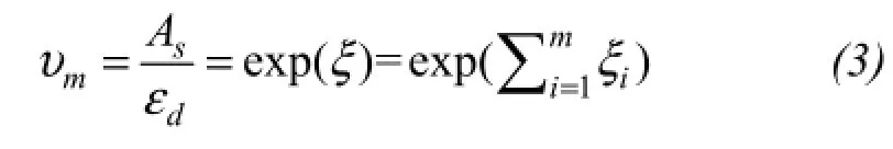
where υmis the attenuation of temperature amplitude in m layers of soil； ξiis the amplitude attenuation in-

dex of ith layer of soil； ξ is the amplitude attenuation index of m layers of soil. ξicould be described by the equation：

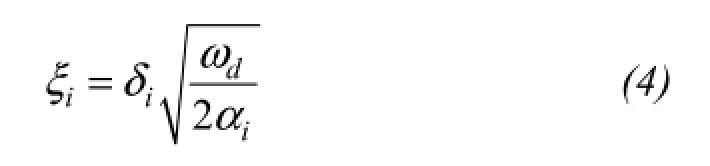
where δiis the thickness in ith layer of soil in subgrade；aiis the thermal diffusivity of ith layer of soil：

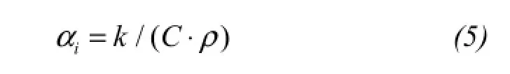
where k is thermal conductivity， W/（m·°C）； C is heat capacity， J/（kg·°C）； ρ is density， kg/m3.

Based on Equation （4）， ξ could be expressed with the equation：

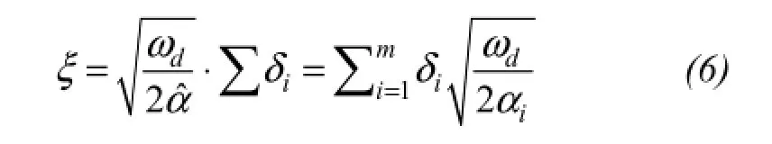
where ∑δiis the thickness of m layers of soil；ˆais the equivalent thermal diffusivity of m layers of soil，which could be described by the equation：

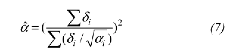
The equivalent thermal diffusivity can reflect the attenuation degree of temperature amplitude through m layers of soil.

3　The calculation method and typical values of the boundary layer thickness

3.1Theoretical solution of the boundary layer thickness

Based on the criteria of boundary layer thickness（Equation （4））， υmis equal to 20 and ξbis equal to 2.996. When the mth layer of soil in subgrade meets the conditions：

The bottom of the boundary layer is in the mth layer of soil and is hbdistant from the top of the mth layer of soil. hbcould be expressed in the equation：

The boundary layer thickness （δu） could be expressed in the equation：

Based on Equation （6）， the boundary layer thickness corresponds to the equivalent thermal diffusivity. The numerical range of the equivalent thermal diffusivity of soil and cushion in subgrade is 2.5×10-7-1.05×10-6m2/s （Xu et al.， 2001）； the numerical range of the equivalent thermal diffusivity of asphalt pavement is 4.3×10-7-8.7×10-7m2/s （Lei，2011； Zhang et al.， 2011）. Thus， the relationship between boundary layer thickness （δu） and equivalent thermal diffusivity （a） could be expressed in Figure 2.

3.2The boundary layer thickness of typical road structure

The typical road includes highway and railroad；the highway pavement structure includes asphalt pavement and cement concrete pavement； the railroad pavement structure includes ballasted roadbed and ballastless roadbed. Based on the design codes and engineering practices （Wang， 2005； Zhang， 2012），four typical embankment structures are widely used in the construction of railway or highway in China， as illustrated in Figure 3. The equivalent thermal diffusivity and the boundary layer thickness of the embankment structures in typical roads is calculated and listed in Table 1.

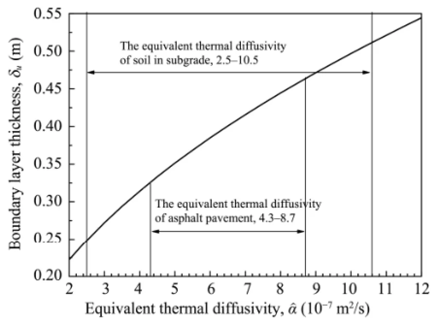
Figure 2　Relationship between δuand aˆ

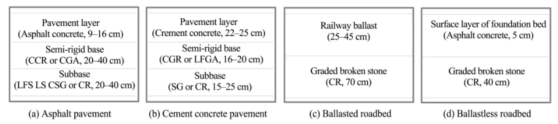
Figure 3　Statistics of embankment structures

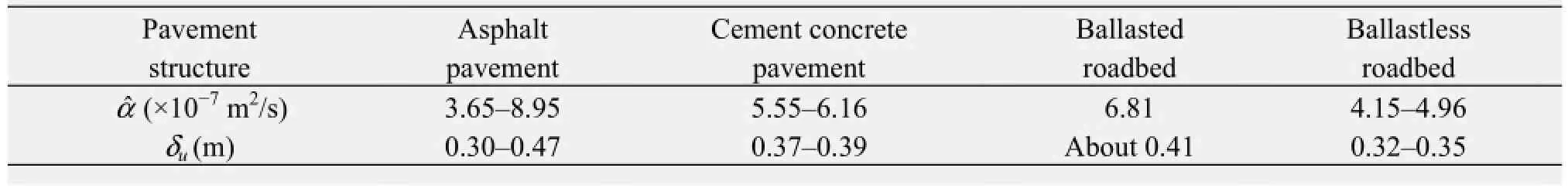
Table 1　Equivalent thermal diffusivity and boundary layer thickness of the embankment structures

4　Determination of the temperature increment with the consideration of local solar radiation condition

4.1The design of the temperature increment of boundary layer

The temperature increment is relevant to the boundary thickness. Bai et al. （2015） put forward that the decisive factor of temperature increment is the effective solar radiation， and the influencing factors of temperature increment are heat-transfer coefficient（B） and equivalent thermal diffusivity （ˆa）. The temperature increment could be designed with the following equation：

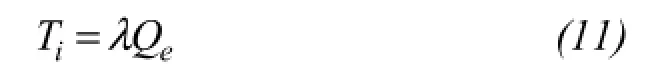
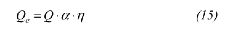
where Qeis the effective solar radiation of one month；λ is the coefficient of temperature increment， which needs to be modified by heat-transfer coefficient and equivalent thermal diffusivity：

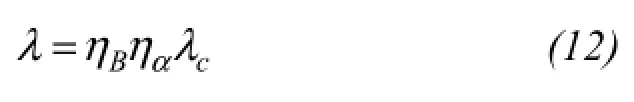
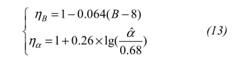
where λcis equal to 0.0090； ηBis the correction factor of heat-transfer coefficient （B）； ηais the correction factor of equivalent thermal diffusivity. ηBand ηacould be expressed with the equation：

where B is heat-transfer coefficient， W/（m2·k）； ˆais equivalent thermal diffusivity， 10-6m2/s.

Based on Equation （13）， the design chart of the coefficient （λ） could be described in Figure 4.

4.2The selection criterion of the factors affecting temperature increment

Obviously， the factors affecting temperature increment include effective solar radiation，heat-transfer of air convection， pavement materials and pavement radiation. The equivalent thermal diffusivity（ˆa） reflects the impact of pavement materials and structure on temperature increment； and ˆa could be calculated by Equation （7） and referred in Table 1.

The heat-transfer coefficient （B） reflects the impact of heat-transfer of air convection on temperature increment. Based on the research of Yan（1984） and Mao et al. （2011）， the value range of B is about 6 to 10 and the empirical formula of B could be expressed in the equation：

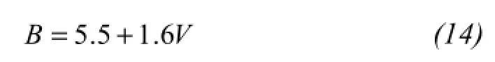
in which V is wind-speed， m/s.

The effective solar radiation of one month （Qe）needs to consider the absorptivity of road surface，road trend and slope angle of road and could be expressed in the equation：

where η is the absorptivity of road surface which could be referred to Table 2 （Qian et al.， 1983）； a is the coefficient of slope angle reflecting the impact of road trend and slope angle on Qe， and a could be referred to Wang （2001）； Q is the measured solar radiation in one month.

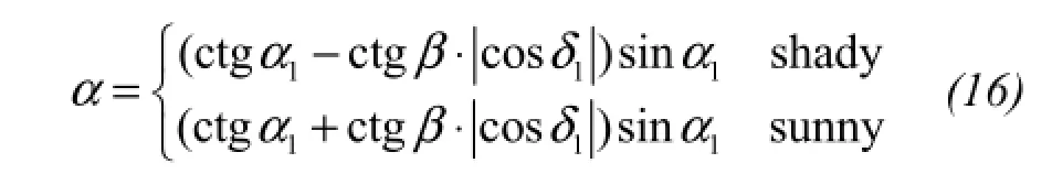
The coefficient of slope angle （a） could be expressed in the equation （Wang， 2001）：where a1is slope angle； β is solar elevation； δ1is road trend angle； for the eastern-western subgrade， δ1is equal to 0°； for northern-southern subgrade， δ1is equal to 90°. When coefficient of slope angle （a） is less than zero， a is equal to 0. The solar elevation could be evaluated in Figure 5.

When the variety of solar radiation in each month is small， Q could be regarded as a constant； or Q could be described in the equation （Weng， 1986； Cha， 1996）：

in which Q0is the average value of solar radiation of each month in a year； Qais the amplitude of solar radiation of each month in one year； with the measured solar radiation in one month， Q0and Qacould be obtained by fitting the least squares principle； ωais the angular frequency， equal to 2π/365d.

When there is a lack of the measured solar radiation， Q0and Qacould be obtained by referring to He and Xie （2010）； the solar radiation of one month could be designed with the equation：

where QAis solar radiation of one month as referred to Figure 6； S is the percentage of sunshine， as referred to Figure 7.

Table 2　Absorptivity of road surface， η

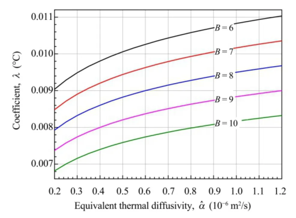
Figure 4　Coefficient of temperature increment λ

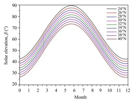
Figure 5　Solar elevation （β）

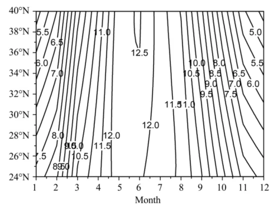
Figure 6　Solar radiation （QA） of one month in Qinghai-Tibet Plateau （×100 MJ）

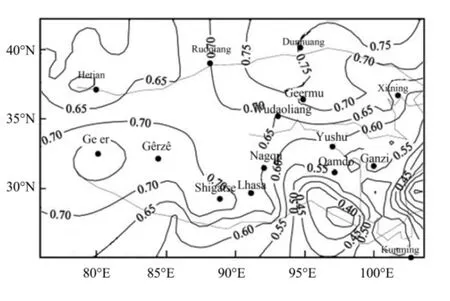
Figure 7　Percentage of sunshine （S） in Qinghai-Tibet Plateau

5　An example of numerical simulation of thermal conduction problem in pavement

5.1The geometric model and material parameters

In a case of the Qinghai-Tibet Highway， subgrade width is 9 m and subgrade height is 2.5 m； the slope angle is π/4 and the geometry model of roadbed is presented in Figure 8. Soil thermodynamic parameters are presented in Table 3 （Cao et al.， 2014）.

The boundary layer thicknesses are listed in Table 4 based on pavement structure and soil layers.

5.2The selection of boundary conditions

In Beiluhe， Qinghai-Tibet Plateau， the latitude is 34.9°N and the longitude is 92.9°E， thus， solar radiation could be designed based on Figures 6 and 7. The absorptivity of pavement， subgrade slope and natural ground are 0.9， 0.7 and 0.6， respectively. The slope angle （a1） is 45°； the angle of the road trend （δ1）is 70.9°； so the coefficient of slope angle （a） could be designed according to Equation （16）. The latent heat（Qw） of vaporization should be deducted from the effective solar radiation. The design of temperature increment （Ti） is expressed in Table 5.

Based on Equation （1）， the upper boundary condition could be described in Equation （19）：

For different position， the parameters could be selected in Table 6.

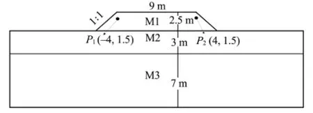
Figure 8　Geometric model

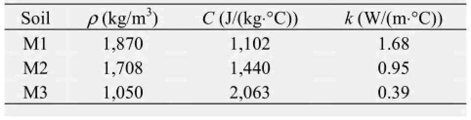
Table 3　Thermodynamic parameters of soils

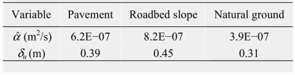
Table 4　Boundary layer thicknesses

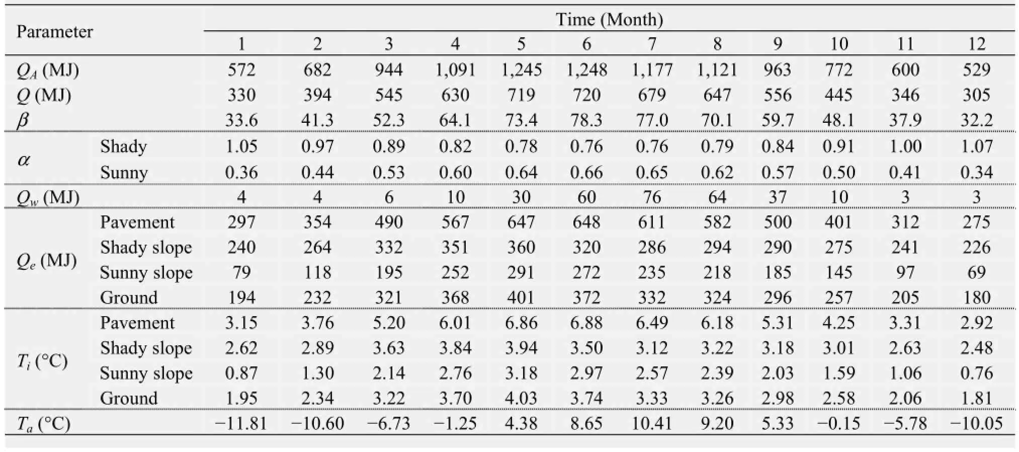
Table 5　Temperature increment

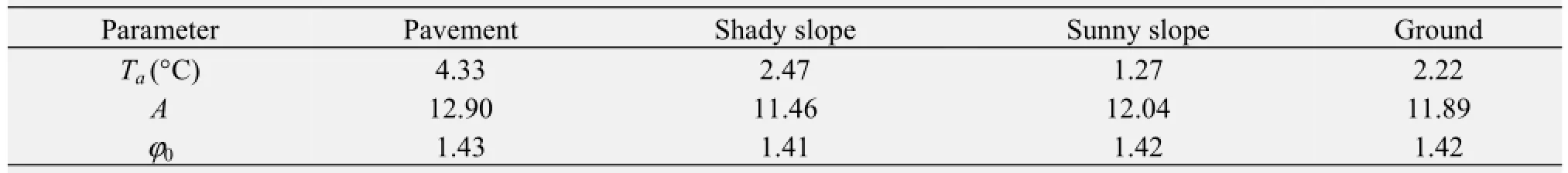
Table 6　Parameters about upper boundary condition of temperature field

5.3Numerical simulation results

The measured value and simulated value of soil temperature at a depth of 0.6 m are listed in Figure 9；and at five years after the subgrade was built， the temperature fields of subgrade in January and July are shown in Figure 10.

As shown in Figure 10， in January， a warming area develops in the subgrade. Based on the comparison of Figure 9， simulated result of temperature field in the subgrade is accurate. According to Figures 8， 10 and 11， the asymmetry of temperature field is not evident and the difference value of temperature in points P1and P2is less than 2 °C. This is because the road trend is 70.9º. In fact， the temperatures in sunny and shady road slopes are related to the road trend. Varying the road trend and maintaining the other simulation settings in upper numerical test， the minimum temperatures of P1and P2（occurring around January）are shown in Figure 11. In Figure 11， when the road trend is 0°， the temperature difference of P1and P2is the largest， about 5.1 °C.

Following the aforementioned procedure， the long term behavior of thermal conduction in any subgrade of highway or railway in permafrost region can be analyzed.

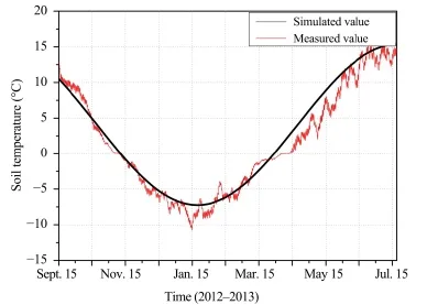
Figure 9　Measured and simulated values of soil temperature at a depth of 0.6 m （in 2012-2013）

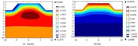
Figure 10　Contour map of temperature field in subgrade （in the fifth year）

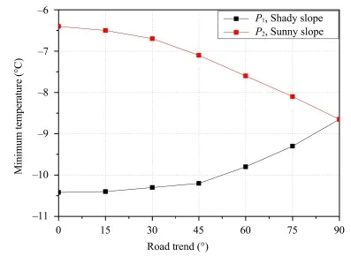
Figure 11　Minimum temperatures of P1and P2in one year with diffident road trends

6　Conclusions

In this paper， a method in the form of equations and design charts is proposed to determine the upper thermal boundary of subgrade where the daily fluctuation of temperature is negligible. The upper thermal boundary of subgrade is determined by two parameters， i.e.， boundary layer thickness and the temperature increment. For typical designs of highway or railway， the boundary layer thicknesses are calculated and listed. Further， the empirical equation and design chart for determining the temperature increment are given in which the following factors are addressed，including solar radiation， equivalent thermal diffusivity and convective heat-transfer coefficient. Using these equations or design charts， the boundary layer thickness and temperature increment can be easily determined and used in the simulation of long-term temperature fields of subgrade.

An example is presented to demonstrate the selection process of the upper thermal boundary in detail and the results prove that the proposed method for determining the upper thermal boundary of subgrade is accurate and practical.

Acknowledgments：

This research is supported by the National Natural Science Foundation of China （Nos. 51378057，41371081， and 41171064） and the National Key Basic Research Program of China （973 Program， No. 2012CB026104）.

Bai QB， Li X， Tian YH， 2015. Upper boundary conditions in the long-term thermal simulation of subgrade. Chinese Journal of Geotechnical Engineering （in press）.

Cao YB， Sheng Y， Wu JC， et al.， 2014. Influence of upper boundary conditions on simulated ground temperature field in permafrost regions. Journal of Glaciology and Geocryology，36（4）： 802-809.

Cha LS， 1996. A study on spatial and temporal variation of solar radiation in China. Scientia Geographica Sinica， 16（3）： 223-237.

He QH， Xie Y， 2010. Research on the climatological calculation method of solar radiation in China. Journal of Natural Resources， 25（2）： 308-319.

Lei XQ， 2011. Determination of specific heat capacity of material（Asphalt， Concrete） for plateau roadbed. Science and Technology， 3： 67-68.

Mao XS， Lu L， Hou ZJ， et al.， 2011. Text and numerical simulation on subgrade temperature field of cement concrete pavement structure. Journal of Chang'an University （Natural Science Edition）， 31（2）： 1-5.

Qian BJ， Wu YW， Chang JF， et al.， 1983. Heat Concise Manual. Beijing： China Higher Education Press.

Wang LJ， 2005. The structure of pavement in west China. Master's Dissertation of Chang'an University， Xi'an， China.

Wang TX， 2001. Research on Calculation Principle and Critical Height of Subgrade in Permafrost Regions. Ph.D. Thesis of Chang'an University， Xi'an， China.

Weng DM， 1986. Climatical method for direct solar radiation calculation and its distribution over China. Acta Energiae Solaris Sinica， 7（2）： 121-130.

Xu XZ， Wang JC， Zhang LX， 2001. Permafrost Physics. Beijing：Science Press.

Yan ZR， 1984. Analysis of the temperature field in layered pavement system. Journal of Tongji University， 3： 76-85.

Zhang HB， Zou L， Ji XP， 2011. Experimental study on the thermal conductivity of asphalt mixtures. Highway， 10： 50-51.

Zhang XD， 2012. Railway Engineering. Beijing： China Railway Publishing House.

Zhu LN， 1988. Study of the adherent layer on different types of ground in permafrost regions on the Qinghai-Xizang Plateau. Journal of Glaciology and Geocryology， 10（1）： 8-14.

Bai QB， Li X， Tian YH， 2015. A method used to determine the upper thermal boundary of subgrade based on boundary layer theory. Sciences in Cold and Arid Regions， 7（4）： 0384-0391. DOI： 10.3724/SP.J.1226.2015.00384.

February 26， 2015 Accepted： May 15， 2015

*Correspondence to： Ph.D.， Xu Li， Associate Professor of Beijing Jiaotong University， Hai Dian District， Beijing 100044， China. Tel： +86-10-51683902； E-mail： cexuli2012@gmail.com