Sensors layout optimization in explosion overpressure field reconstruction

WANG Feng， BAI Yuan-qi

(School of Information and Communication Engineering, North University of China, Taiyuan 030051, China)



Sensors layout optimization in explosion overpressure field reconstruction

WANG Feng， BAI Yuan-qi

(SchoolofInformationandCommunicationEngineering,NorthUniversityofChina,Taiyuan030051,China)

The paper proposes four indicators to guide sensors layout in practical experiment on explosion overpressure filed construction based on tomographic method with high reconstruction accuracy and the least sensors. First, genetic algorithm is adopted to conduct global search and sensor layout optimization method is selected to satisfy four indicators. Then, by means of Matlab, the variation of these four indicators with different sensor layouts and reconstruction accuracy are analyzed and discussed. The results indicate that the sensor layout method proposed by this paper can reconstruct explosion overpressure field at the highest precision by a minimum number of sensors. It will guide actual explosion experiments in a cost-effective way.

explosion overpressure field; genetic algorithm; sensor layout optimization; travel time tomography

0 Introduction

Explosion technology includes underwater explosion, air explosion, underground explosion, etc. It is widely in the fields of seismic exploration, mines, drilling, national defense, and so on. However, explosion process is violent and quickly, it is difficult to directly measure the explosion overpressure of the whole shock wave. Generally, the points test with the aid of a variety of sensors is made to estimate explosion performance and power as well as tomographic technology is used to reconstruct explosion overpressure field. However, the explosion experiment based on sensors is expensive and complex, especially for a devastating explosion experiment, the sensors will not be used again. Considering experiment cost, it is essential to select the sensors as few as possible and simultaneously to propose an optimal sensors layout scheme[1].

The purpose of this paper is to propose practical and concrete optimization index and constraints, use reasonable optimization algorithm to determine the number of sensors, makes an optimized sensor layout by programming, and reconstruct the explosion overpressure filed with the least sensors, low cost and high reconstruction accuracy.

Although there exist many sensors layouts, lisuch as spiral type, concentric type, etc.[2], they may not be suitable for overpressure field reconstruction. This paper proposes four indicators to guide sensors layout in practical experiment on explosion overpressure filed construction based on tomographic method using global search with high reconstruction accuracy and the least sensors[3-4]. The proposed method generates a better distribution station program and has good military applications.

1 Tomographic method

This paper uses tomographic method to reconstruct explosion overpressure field.Msensors are laid around the center point of bomb. After blasting, shock waves spread from the center point to theMsensors and thenMpropagation path rays are formed. According to the shock wave transmission law, the reconstructed area is divided intoNdiscrete irregular grid cells in accordance with the shockwave attenuation law, as shown in Fig.1.

Assume that the shock wave is transmitted not along the boundary of the grid cell but along a approximately straight line within each grid cell, with each sensor corresponding to a ray. Travel time is that in which shock wave arrives at the sensor and it is the function about speed and geometric path as described by

whereris ray,vis speed,sis the reciprocal of velocity and is called slowness, andLis integral path.

Fig.1 Explosion shock wave propagation model

Discretize the above equation according to the test area meshing, for rayi, the travel time is described as

wheretiis the travel time of rayi;dij, the length of rayipassing throughj-th grid ray;sj, slowness in thej-th grid cell;m, the number of rays; andn, the number of grid cells.

The above equation can be written in matrix form as

whereT=[t1,t2,…,tm]Tism-dimension column vector consisting ofmdiscrete travel times;S=[s1,s2,…,sn]TisN-dimension column vector consisting ofNunknown discrete slowness values; andDis a sparse matrix, whose elements aredij.

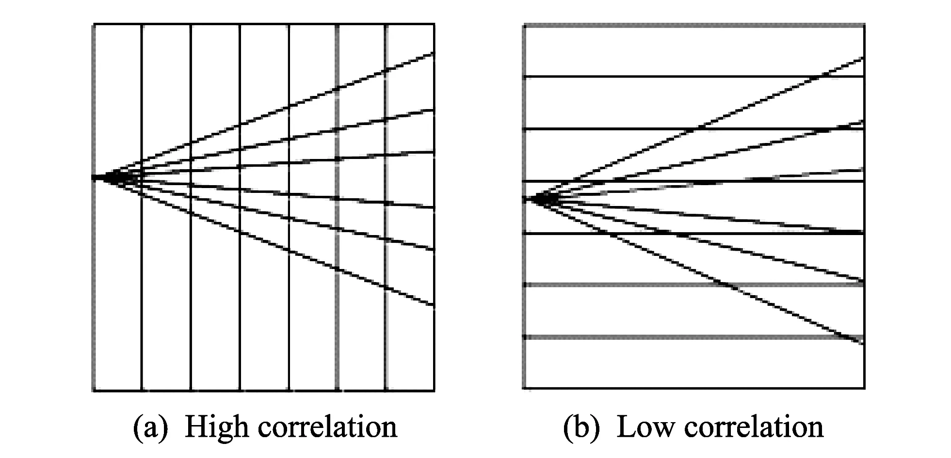
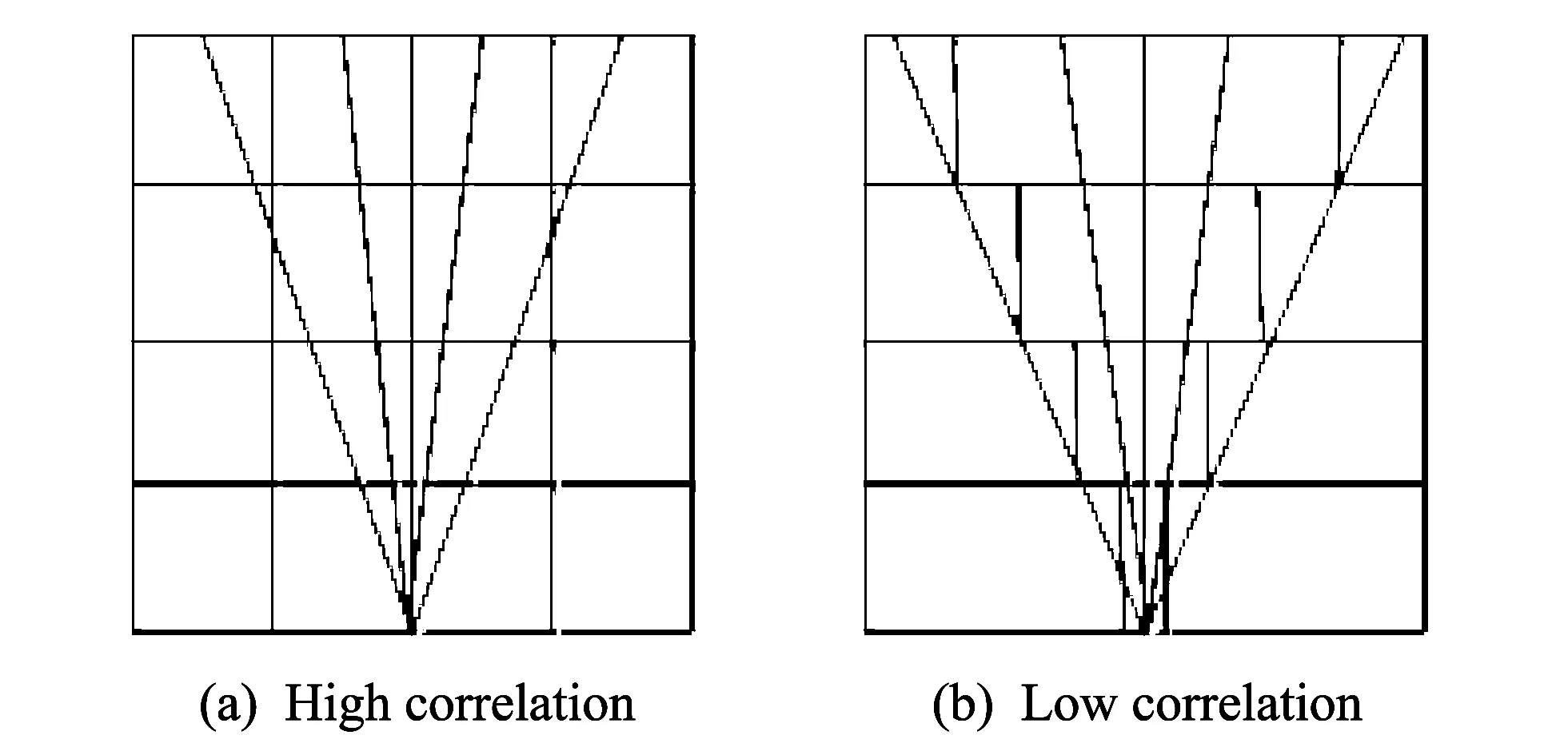
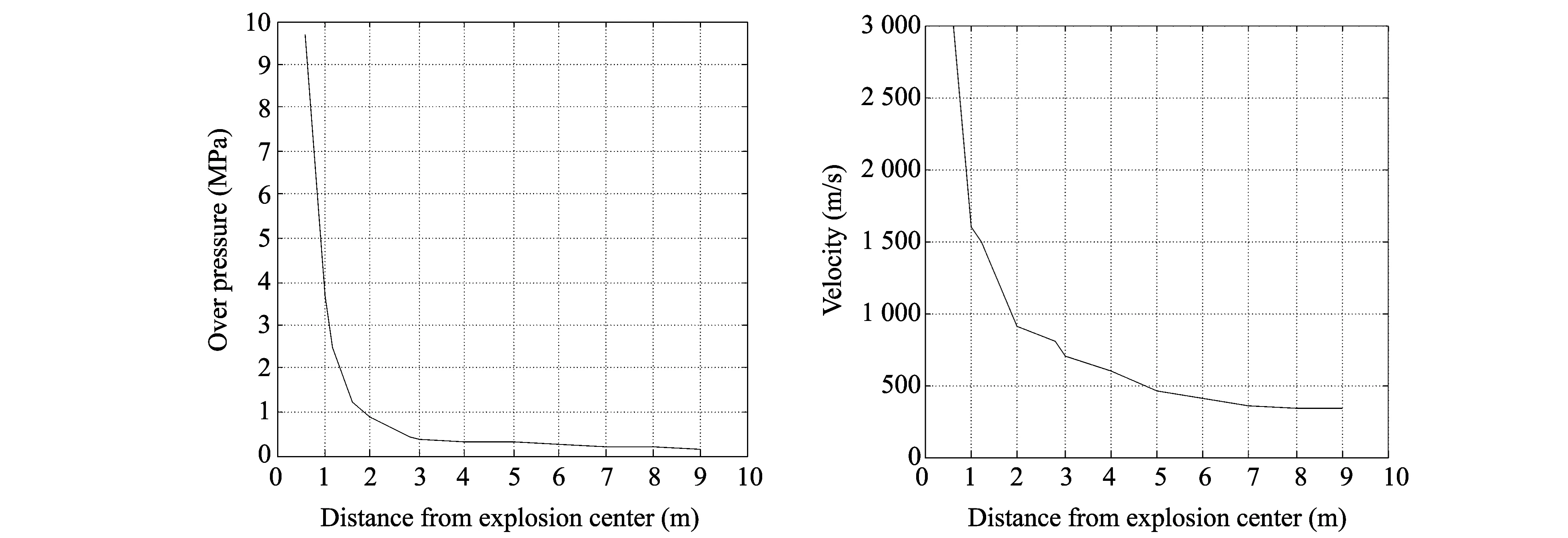
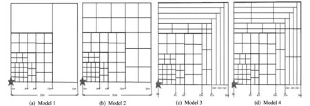
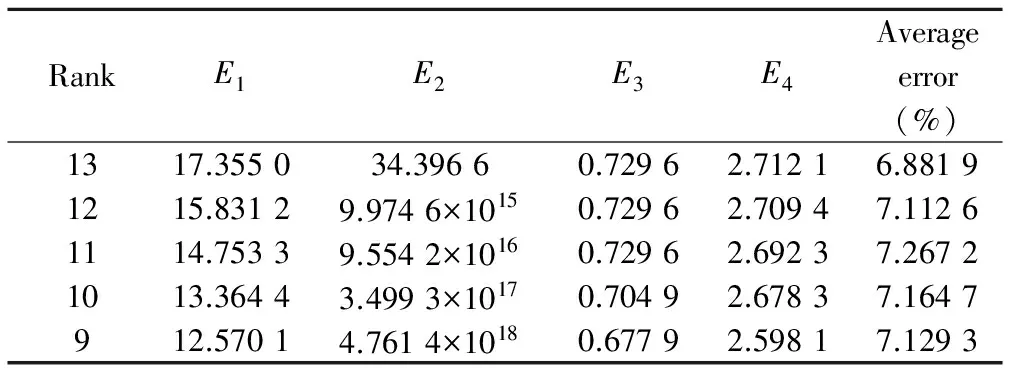
D∈Rm×nis the“tomographic matrix” withn

2 Layout guidelines

2.1 Rank and eigenvalues

Solving Eq.(3) is actually seeking the inverse matrix of coefficient matrixD. However, for this inversion problem of single explosion source, coefficient matrixDis generally singular.Since we need to solve the problem using the generalized inverse theory, the singular value decomposition (SVD) ofD∈Rm×ncan be written as

The greater the rank and the larger the singular values ofD, the stabler the inversion problem and the more independent information may be gained from the data. Now, we can define measurement stability to be maximized as the sum of the normalized singular values and the rank (r) ofD. Since the singular values ofDare the positive square roots of the eigenvalues ofDTD, the stability index ofD, namely the cost function, can be defined as

wherenis the number of the model cells;Pis the rank ofD;λ1denotes the maximum eigenvalue ofDTDandλidenotes the whole eigenvalue.E1consists of two parts: the first part reflects the relative distribution of singular values, and the other part reflects the quasi-null space. The cost functionE1has the max mum and any increase inE1results in a better conditionedDwith smaller quasi-null space[5-6].

2.2 Condition number of equations

Stability of Eq.(3) depends on the condition number of the coefficient matrixD. The larger the condition number, the worse the stability problems, and vice versa[7]. If the observed data from obtainedThave minor changeδT, defining the change in the solution asδS, then Eq.(3) is written as

D(S+δS)=T+δT,δS=D-1δT.

Accordingtothenatureofthenorm

‖δS‖≤‖D-1‖‖δT‖, ‖T‖≤‖D‖‖S‖,

Then

wherecond(D)=‖D‖‖D-1‖ is the condition number of matrixDon the solution of the equation.When the coefficient matrixDhas errorδD, it can be got as

(D+δD)(S+δS)=T,

ForthecoefficientmatrixDwith errors, the relative error of equations still depends on the size of the condition number.So the condition number of the solution is an important indicator to evaluate the quality of the equations. The greater the condition number, the severer ill-posedness it has.Therefore, the conditions number is defined as the second evaluation criteria as

E2=cond(D).

2.3 Ray density and orthogonality

Ray density denotes the number of rays passing through per image of every grid. The main factors that lead to the existence of zero-space solution of equations are those rays not passing through the grid cell.Since the ray density is increased, which can lead to the increase of non-zero elements of the matrixD, the matrixDis equal to zero vector to avoid a column vector. Ray orthogonality is defined as the cosine of the largest angle between rays covering each grid cell.

In this paper, ray density and ray orthogonality are defined as

whereRay_densityjis the density of each grid cell；mis the total number of rays；nis the total number of grid cells; andsjis the area of grid cell.

Ray_orthogonalityj=sin(max(θ)),

whereRay_orthogonalityjis the density of each grid cell andθis angle of all rays covering each grid cell.

The smaller the ray density region and the less the poor orthogonal, the larger the inversion[8]. Therefore, the average radiation density and average radiation orthogonality are defined as the layout guidelines,

If the mathematical values ofE3andE4are smaller, the inversion errors would be much greater. When laying the sensor, we should make ray coverage wide and distribute it evenly to reduce the number of zero elements of the matrix and condition number.

3 Model strategy

3.1 Meshing principle

Based on the above analysis, the model strategy of rebuilding region directly affects the layout optimization of the sensor. For the regional model strategy, we must fully consider the coefficient matrixDlinear correlation and select the appropriate reconstruction model[9].

As shown in Fig.2, six sensors have the same layout. If we select the model in Fig.2(a), only three valid equations could be established. Because this model allows the upper and lower sensors to be distributed in ray linear correlation, if it is replaced by the model in Fig.2(b), all six equations could be established.

Fig.2 Rectangular net model

The concentric model is shown in Fig.3.

Fig.3 Concentric model

Fig.4 Complex grid model

The sensor distribution is linearly correlative in Fig.3(a), which reduces the number of equations. However, the model in Fig.3(b) makes theDbe unrelated to uncertainty reduction. As Fig.4(a) shows, according to the regular 4×4 mesh rule, four rays go through the grid with equidistance, thereforeDwill be an approximately linear correlation. If it is replaced by the model in Fig.4(b), an irregular grid, it can be unrelated.

3.2 Sub-region multi-scale grid

In the explosion, the empirical formula of shock wave peak overpressure variation with distance has many forms. Its attenuation wave form is shown in Fig.5. Although there is difference in the calculation results of the empirical formula, it can be seen that, in the near field region, the overpressure decreases rapidly. As the proportion of distance increasing, peak overpressure gradually decreases, and finally levels off. If a uniform rectangular grid is used throughout the region, which will result in large errors in the explosion source region, where overpressure and speed change rapidly. Therefore, when reconstructing the peak overpressure field and the velocity of shock wave, not a single scale grid but a multi-scale grid should be adopted according to overpressure and velocity attenuation law.

Based on the distance from the explosion center, the entire reconstruction area is divided into different sub-regions, and different mesh sizes are used in different sub-regions. In the near field region, overpressure decays faster, the fine mesh method is used and the distribution grid mesh size is small and dense; coarse mesh method is used in the far field region with large mesh size and sparse. To avoid some linear correlation of row vectors of matrixD, different grid scales are also used in a symmetric region. Such programs can be a good reaction on overpressure attenuation characteristics. However, if there is a big gap between the maximum and the minimum mesh sizes of the grid, due to the nature of the error propagation, large errors will be introduced. For example, in Fig.(2),mrays are used to establish the equation as

Considering the algorithm and other reasons, each reconstruction speed in Eq.(12) will produce some errors, i.e.x1→ξ1,x2→ξ2,…,xn→ξn. Therefore, the total error ofmrays is

namely,

tm=|Dξ|>|ξ|.

Itcanbeconcludedthat,ifthemeshsizeandmeshraylengthdijare larger, the produced error becomes larger. Meanwhile, too large difference between mesh cells will produce larger initial error. The mesh used in the test should be based on the number of sensors, meeting both tomography resolution and accuracy requirements[11].

Fig.5 Shock wave attenuation with distance

3.3 Model tests

According to the above analysis, the overpressure field in the range of 90° is reconstructed, as shown in Fig.6. Taking different models, the changes of the reconstruction accuracy can be observed.

Fig.6 Different sub-region multi-scale models

For each model, Table 1 lists the maximum and the minimum mesh sizes, average mesh size and reconstruction error.

Table 1 Influence of mesh size on reconstruction

The model 3 is more reasonable becasue the gap between the mesh cells is smaller and the reconstruction error is minimized. Thus this paper selects model 3.

4 Simulation

4.1 Sensors layout with D full rank

Considering the above models, the layout of the sensors must ensure that each grid is passed by at least one ray, so that the problem is solvable. Based on this, the position of the sensors is adjusted to improve Eq.(3) .

Take 13 sensors for example, the positions of the sensors are arbitrarily changed and the each index of coefficient matrixDunder different layouts is obtained. Analyzing the results from the proposed indicatorsE1,E2,E3,E4and the eigenvalues, the errors above are reconstructed and the regularity between different sensors layout and these indicators can be observed.

Fig.7 Eigenvalues distribution of 13 sensors under different layouts

In Fig.7, each curve represents the distribution of eigenvalues in a particular rankp, whereprepresents the rank ofDDT. Ifp=13,Dis full rank, or elseDis dissatisfied with the rank distribution and there is a linear correlation vector inD.

When 13 sensors are distributed by full rank, namelyp=13, the eigenvalues ofDDTis 13. When 13 sensors are distributed by dissatisfied rank, the number of eigenvalues are less than 13, and the eigenvalues are less than full rank. With five curves descending successively from the top to the bottom, the eigenvalues reduce successively, which means that with the rank decreasing, their eigenvalues are reduced .

It can be observed from Table 2 that with the rank decreasing,E2increases sharply.E2is 34.396 6 in full rank and it dissatisfies the rank with squared magnitude of 1015, which means that the equation becomes increasingly unstable. BecauseE1,E3andE4are smaller, the mathematical properties ofDget worse, and the error becomes bigger and bigger.

In summary, the above four indicators directly affect the reconstruction accuracy. When it dissatisfies the rank, adjusting the sensors layout can make the matrixDbe full rank; Reducing the condition number of equations can improve ray coverage and make the equation relatively stable, thus the reconstruction accuracy can be improved.

Table 2 Variation law of indicators for 13 sensors under different layouts

RankE1E2E3E4Averageerror(%)1317．355034．39660．72962．71216．88191215．83129．9746×10150．72962．70947．11261114．75339．5542×10160．72962．69237．26721013．36443．4993×10170．70492．67837．1647912．57014．7614×10180．67792．59817．1293

4.2 Adjustment of sensors layout

The maximum linearly independent group of vectors is not unique, but its vector number in every great maximum linearly independent group is unique. The rank of the matrix is the number of vectors in its row or column vectors’ maximum linearly independent group. Therefore, the rank of a certain matrix can be determined by the maximum linearly independent group of vectors. In view of the link of the maximum linearly independent group and the rank, it often “borrows” the maximum linearly independent group to solve the problem of the rank of the vector group.

In this paper, we obtain stair matrices by elementary row of matrixDT, which is the transport matrix of coefficient matrixD. Then observe each stair sub-type of the stair matrices, adjust the position of the corresponding sensors, and makeDfull rank. As Fig.8(a) shows, it is a distribution of 13 sensors. In this arrangement, the rank of the coefficient matrixDis 12, which shows that the layout of two-sensor locations makes the elements of the composition of the two lines be linearly related. By elementary row translation of matrixDTto obtain stair matrices, it can be observed that the first and the second rows of the matrices are laid on the same ladder, which means that No.1 and No.2 sensors are distributed incorrectly to dissatisfy the rank. At the same time, it is found that the two sensors pass through the same number of grids, which results in the linear correlation.

Adjusting the position of one sensor to eliminate linear correlation, full rank distribution is obtained, as shown in Fig.8(b).

Fig.8 Sensors layouts adjustment

4.3 Sensors layout optimization

To optimize the layout of the sensors for explosion field reconstruction, the number of sensors should be reduced from 13 sensors based on genetic algorithms until a smaller number of sensors cannot be found to reconstruct the model. The results are shown in Fig.9.

Fig.9 Eigenvalues distribution of different sensor numbers

As Fig.9 shows, the eigenvalues of matrixDDTare distributed at different sensor numbers. Each group of sensors are full rank. The curve (13 sensors) is located at the top and is the longest, which means the eigenvalues of 13 sensors are the largest and the most. With the reduction of the number of sensors, the eigenvalues are reduced and become smaller. This trend describes that the more sensors, the larger and much eigenvalues. The behavior of equation is better and the solution is relatively stable.

Table 3 Variation law of indicators for different sensors

As Table 3 shows, with the sensors decreasing, indicatorsE1andE4gradually decrease. This indicates that mathematical properties ofDare getting worse, and ray density and orthogonality become smaller. Using fewer sensors, the reconstruction errors will be large and the results will be worse.

The simulation shows that at least five sensors are needed to cover each grid cell in this model.As shown in Table 3, when there are 13 sensors, the reconstruction error is 6.876 8%. When there are 5 sensors, the reconstruction error is 7.794 6%. As the number of sensors is reduced, the average error becomes larger and larger. Therefore, reconstruction accuracy depends on the number of sensors largely.

5 Conclusion

First of all, a scheme of explosion overpressure field reconstruction is put forward in this paper. Based on this scheme, we adopt the sub-region multi-scale model strategy for explosion overpressure field. Secondly, for explosion overpressure field reconstruction, the paper proposes four indicators to guide the optimization layout of sensors by programming. Finally, the conclusions are as follows:

1) Sub-region multi-scale mesh model can meet different resolution requirements of near field, midfield and far field. It has strong anti-interference ability and uses the least sensors.

2) When arranging the sensors, the rank of ray path matrix should be bigger, similarly for characteristic value, ray density and ray orthogonality. The fewer the condition number, the better the sheme.

3) For the layout with the same number of sensors, a distribution needs to be found and makes the ray path matrix be full rank, which can reduce the number of condition equations and increase ray density. Thus the equation is relatively stable and the reconstruction accuracy is improved. If it is dissatisfied with the rank distribution, we can adjust the position of the sensors according to the maximum linear independence of ray paths matrix for optimal layout.

4) Reconstruction accuracy is largely dependent on the number of sensors. In actual test, we save the cost at the expense of reconstruction accuracy by reducing the number of the sensors used. To achieve high precision, we need to increase the sensors.

5) Combined with the actual situation, in the real experiment, the four indexes proposed in this paper are used to establish the appropriate fitness function. By using genetic algorithm, we can find out the minimum number of the sensors needed and the optimization of layout program to save the experimental cost.

[1]LIU Yan, LIU Gui-jie, LIU Bo. Research status and prospect on optimal placement of sensor. Transducer and Microsystem Technologies, 2010, (11): 4-6.

[2]ZHOU Lei. Optimal disposition of multi-sensor based on genetic algorith. Chengdu: Univercity of Electronic Science and Technology of China, 2012.

[3]TANG Fei, TENG Hong-fei. A modified genetic algorithm and its application to layout optimization. Journal of software, 1999, 10(10): 1096-1102.

[4]HUANG Liang. Methodology and experiment research on concrete ultrasonic computerized tomography. Hu’nan: Hunan University, 2008: 5.

[5]Wéber Z. Optimizing model parameterization in 2D linearized seismic traveltime tomography. Physics of the Earth and Planetary Interiors, 2001, 124(1): 33-43.

[6]Curtis A, Snieder R. Reconditioning inverse problems using the genetic algorithm and revised parameterization. Geophysics, 1997, 62(5): 1524-1532.

[7]CHENG Gu. Theory and application of seismic reflection tomography when walking. Shanghai: Tongji University, 2004.

[8]Passerini C, Falciasecca G. Modeling of orthogonality factor using ray-tracing predictions. IEEE Transactions on Wireless Communications, 2004, 3(6): 2051.

[9]Vesnaver A. Null space reduction in the lineearized tomographic inversion. Modern Approaches in Geophysics, 1995, 12: 139-145.

爆炸超压场重建的传感器布局优化

王 凤， 白原齐

(中北大学 信息与通信工程学院， 山西 太原 030051)

本文提出了4个指导传感器分布的指标， 结合走时层析成像技术重建爆炸超压场， 在满足重建精度的前提下最大程度地减少传感器数目。 首先采用遗传算法全局搜索出满足这4个指标的传感器的分布方案； 然后通过MATLAB模拟仿真， 并对不同传感器布局方式下这4 个指标的变化规律及重建精度进行了分析和讨论； 结果表明， 采用本文所提出的传感器分布方案可以用最少数目的传感器重建出最高精度的爆炸场， 进而为实际爆炸试验节省费用。

爆炸超压场; 遗传算法; 传感器优化布局; 走时层析

WANG Feng， BAI Yuan-qi. Sensors layout optimization in explosion overpressure field reconstruction. Journal of Measurement Science and Instrumentation, 2015, 6(4)： 307-314.

10.3969/j.issn.1674-8042.2015.04.001

Foundation item： Natural Science Foudation of Shanxi Province of China (No.2013011017-8)

WANG Feng (1102653569@qq.com)

1674-8042(2015)04-0307-08 doi： 10.3969/j.issn.1674-8042.2015.04.001

Received date： 2015-09-11

CLD number： TP212.9 Document code： A