Spatial pattern analysis for quantification of landscape structure of Tadoba-Andhari Tiger Reserve, Central India

Ambica Paliwal • Vinod Bihari Mathur

Introduction

The management of wildlife and protected areas has several goals: conservation, optimal use of forest resources, meeting the demands for the scientific underpinnings of managing landscapes,and incorporating the consequences of spatial heterogeneity. The sensitivity of ecological effects of resource management towards spatial configuration is gaining acceptance worldwide. The land cover classification from remote sensing data is a powerful tool that can provide repetitive and spatial information concerning the landscape (Chust et al. 2004).

Studies have highlighted the role of remote sensing data from earth observation satellites in forest ecology (Jadhav et al. 1990;Innes and Koch 1998; Skole and Tucker 1993 and Franklin et al.1994). Satellite remote sensing plays a crucial role in generating information about forest cover, vegetation types and land use changes (Cherill and McClean 995). Both coarse and fine spatial resolution satellites have proved to a significant resource for forest mapping. Milanaova et al. (1999) studied broad vegetation type stratification using coarse resolution data like NOAAAVHRR and several studies have also reported mapping at finer resolution data of LANDSAT TM+ (Groom et al. 1996; Guillem et al. 2004). Remote sensing estimates of regional variation in biodiversity can be used in analyzing diversity patterns, landscape patterns and aiding conservation efforts (Gould 2000).Spatial patterns have a strong influence on the information content of ecosystem components. Since landscape structure is often regarded as an important pre-requisite that governs the distribution and abundance of species, the first step is to understand landscapes and their dynamics. It is widely acknowledged that patterns of landscape elements strongly influence the ecological characteristics. Therefore, spatial pattern characterization and quantification of land-cover classes to relate pattern and process is a pre-requisite at landscape level (Turner 1987). It is not only important to understand how much there is of a particular com-ponent but also how it is arranged (Turner 2001). Quantification of landscape pattern is necessary for understanding the composition and configuration of landscapes. The underlying premise is that the explicit composition and spatial form of landscape mosaic affect ecological systems in ways that it would be different,if the mosaic composition or arrangement were different (Wiens 1995). Moreover, recent studies have demonstrated that land use and landscape changes significantly affect biodiversity (Cousins and Eriksson 2002; Gachet et al. 2007; Miyamoto and Sano 2008). Spatial tools of remote sensing and GIS have a capacity to quantify land-cover patterns and understand spatial heterogeneity(Turner 1990; Sinha and Sharma 2006). Methods are needed to quantify aspect of spatial patterns that can be correlated with ecological processes (O’Neill et al. 1988).

A large number of spatial indices are based on patch metrics that quantify the spatial pattern at three different levels of organization—patch, land cover, and landscape—using the programme FRAGSTATS (McGarigal and Marks 1995). Numerous studies have advocated the authenticity of this spatial pattern analysis programme (Lu et al. 2003; Cushman et al. 2008; Lele et al. 2008). The landscape structure of the U.S. state Kansas was analysed at three scales by calculating the landscape pattern metrics (Griffith et al. 2000). The utility of landscape pattern indices was studied for judging the habitat implications of alternate landscape plans or designs (Correy et al. 2005). LISS III data of IRS 1D and IRS P6 were studied and compared for landscape ecological application by computing class level and landscape level metrics (Sharma 2009).

Previous studies conducted in the study area (Dubey & Mathur 1999; Dubey 1999) were restricted to the classification of vegetation using IRS LISS II data of 36.5m coarse resolution. However, neither of the studies have ever dealt with exploring the landscape structure of TATR. Satellites with high spatial resolution facilitates detailed assessment of vegetation, identification of smaller patches and is also considered helpful in evaluation of impacts on biodiversity of specific management policies (Innes and Koch 1998). IRSP6 LISS IV is one such high resolution satellite. Several studies have assessed the utility of LISS IV in different thematic areas: Gupta and Jain (2005) carried out urban mapping; Kumar and Martha (2004) assessed damage from landslide; Rao and Narendra (2006) mapped and evaluated urban sprawling; Kulkarni et al. (2007) studied glacial retreat in Himalaya; and Bahaguna (2004), Sarangi et al. 2004; Rajankar et al.(2004) evaluated application of IRS P6 in coastal and marine zones. Since this satellite it is expected to provide a new opportunitiesy to efficiently make detailed vegetation cover maps efficiently for large study areas, the present study was initiated with the aim to document and map the current status of the TATR forest. The IRS P6 LISS IV data was of 5.8 m high resolution and was used to describe the landscape structure of TATR at three spatial levels of organization: viz. landscape level, class level, and patch level. The primary objective of thise study is to understand the habitat quality of TATR for better conservation management of the tiger reserve for large mammals by providing general characterization of the landscape structure and patterns.

Materials and methods

Study area

The Tadoba-Andhari Tiger Reserve (TATR) represents an important habitat for wildlife in Maharshtra State in Central India.It comprises of Tadoba National Park (TNP) and Andhari Wildlife Sanctuary (AWLS).The area lies between 20°04' to 28°025'N and 79°13' to 79°33'E (Fig.1). It covers 625.40 km² and has a subtropical climate with three distinct seasons: summer, monsoon, and winter. The climate is characterized by a hot and prolonged summer while winter is short and mild. TATR is mostly undulating and hilly in the north and almost a plain in the southern part of the TATR. It has been classified as southern tropical dry deciduous forest (Champion and Seth 2005).

Data source

Three digital scenes of IRS-P6 LISS IV with 5.8m resolution were acquired from the National Remote Sensing Agency(NRSA) for December 2005 and January 2006. During this period the vegetation was in full bloom and cloud free data could be obtained.

Data analysis

Image preparation for classification

Unwanted artefacts like additive effects due to atmospheric scattering were removed through set of pre-processing or cleaning up routines. First-order radiometric corrections were applied, using the dark pixel subtraction technique (Lilesand & Kiefer 1994).This technique assumes that there is a high probability that at least a few pixels within an image should be black (0% reflectance). Because of atmospheric scattering, the imaging system records a non-zero Digital Number (DN) value at the supposedly dark- shadowed pixel location. Therefore the DN value was subtracted from the data to remove the first-order scattering component. Images were then registered geometrically. Uniformly distributed Ground Control Points (GCPs) were marked with a root mean square error of less than one pixel and the image was resampled by the nearest neighbourhood method. All the scenes were mosaiced and the study area was extracted using digital boundaries. A reconnaissance survey was conducted from February–June 2006 to have gain an overview of broad vegetation types in the study area and to devise a sampling strategy for detailed sampling analysis. An approach of systematic stratified sampling was used and range maps were used developed to stratify the area for ground-truthing and vegetation plots. Later, from June 2006 to February 2008, intensive ground- truthing was conducted and a total of 810 GPS points, including 520 vegetation plots, were collected to capture the variation in spectral signatures of different vegetation types over the entire study area and to achieve higher accuracy of vegetation mapping. Some 810 spectral signatures were collected out of which 284 were used forthe accuracy assessment. The data collected from the plots was subjected to hierarchical cluster analysis to determine the vegetation communities existing in the field.

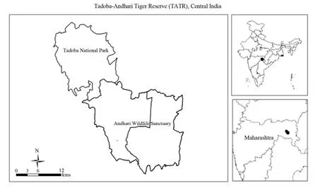
Fig.1. Study area

Image classification

Unsupervised classification was done on image, using the nearest-neighbour algorithm for differentiating spectral reflectance of various objects (Lilesand and Kiefer 1994). It examines the similar pixels in an image and aggregates them into a number of classes. Initially, the entire area was classified into 40 classes,which were iterated 10 times with convergence threshold of 0.98.According to Champion and Seth (2005), the area is classified under group 5 and subgroup 5A as Southern Tropical Dry Deciduous Forest. The entire area was divided into 40 classes initially. Later, these 40 classes were classified under the broad er classes of forest, waterbody, scrub, open forest and agriculture/settlement. The non-forest classes were masked and cluster analysis was conducted on the data acquired from vegetation plots to determine the forest communities. Results of cluster analysis were then used to classify forest classes. Finally, 40 classes were merged into 10 classes, including six vegetation classes which were well observed on the ground. The pixellated classified output image was obtained. Since the objective of the study is to study habitat quality of TATR for large ungulates,therefore, map was subjected to two 3×3 filters to ensure smoothening and the patches below 0.5ha were removed. Area of 0.5 ha was considered as insignificant to study habitat of large ungulates. Finally, the area was calculated for each class. The accuracy of the map was tested using some of the ground truth points not used during classification. The land cover information of these locations was compared to classified maps. Accuracy was tested using Kappa Statistics (Khat coefficient) (Lillesand and Kiefer 1994).

Image preparation for Fragstats

For Fragstats input, rasters 0s (background data) was recoded as negative integers so that it would be ignored by Fragstats.

Landscape structure analysis

For the quantification of the TATR landscape of TATR, uses of statistical measures or indices were made that describe landscape configuration and composition. These indices were calculated by FRAGSTATS (Mcgarigal and Marks 1995). The FRAGSTATS is a spatial pattern analysis programme for categorical maps. It simply quantifies the areal extent and spatial configuration of patches within landscape. There are two versions of FRAGSTATS, Vector (ARC/INFO) and Raster (Image Maps) versions.The raster version has been used in this study to compute metrics.The landscape structure was analyzed at three different spatial scales, viz., landscape, class and patch levels, using 12 sets of indices as shown in Table1. The reason to selected these indices were attributed to their simplicity. These were the basic indices,which provided the general description of the landscape. Numerous studies have supported their authenticity of these indices(Griffith et al. 2000 and Cushman and Neel 2008). Fig.2. de- scribes the methodology in the form of a flow chart.

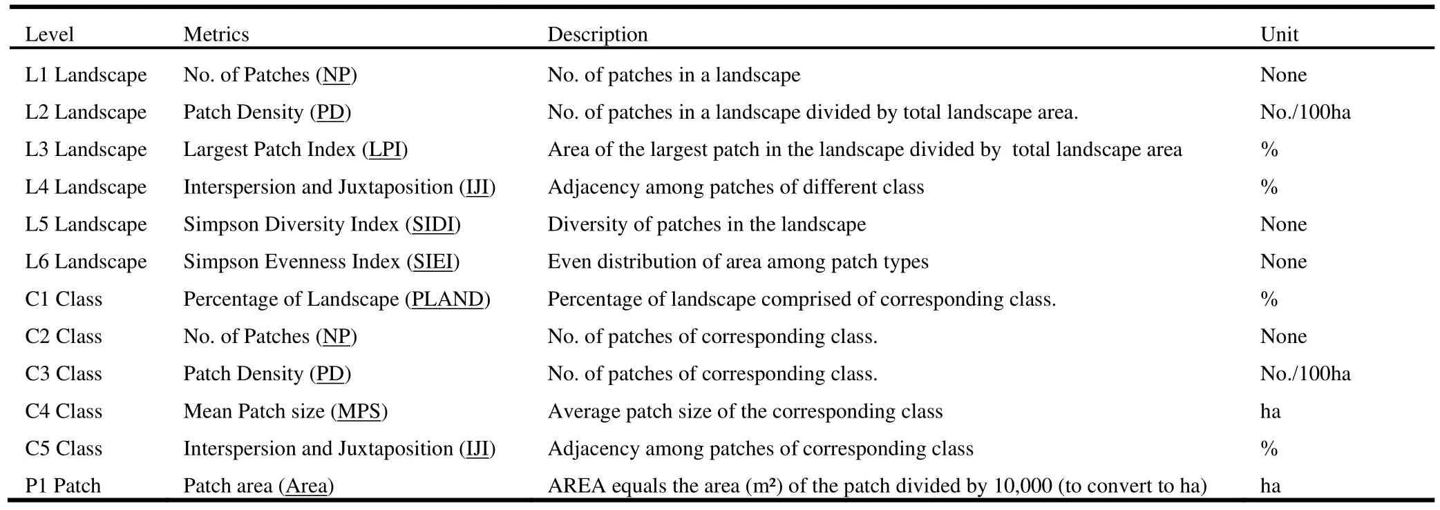
Table1. Metrics used for the landscape characterization of TATR

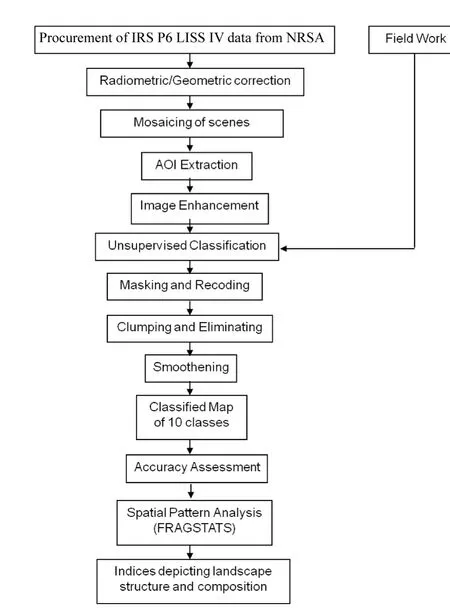
Fig.2. Flowchart of methodology

Results

Landscape composition

Seven communities were identified from cluster analysis: Tectona, Tectona-Cliestanthus, Tectona-Chloroxylon, Zizyphus-Adina, Pterocarpus-Flacourtia, Dalbergia-Mitrigyna and Riparian community. Mapping was done using the cluster analysis as a premise (Fig.3). As a result, 10 landcover/landuse classes were delineated: teak forest, teak mixed bamboo forest, mixed forest,mixed bamboo forest, riparian forest, grassland, scrub, open forest, agriculture/settlements and water body (Fig.4). Amongst the vegetation classes, mixed bamboo forest occupied the maximum proportion of the study area (75.81%) and the riparian forest occupied the least (0.61%). Table2 shows the areas of the different classes mapped.

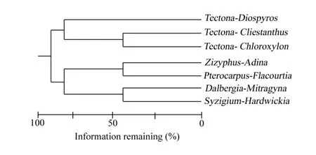
Fig.3. Dendrogram showing the different communities using hierarchical cluster analysis

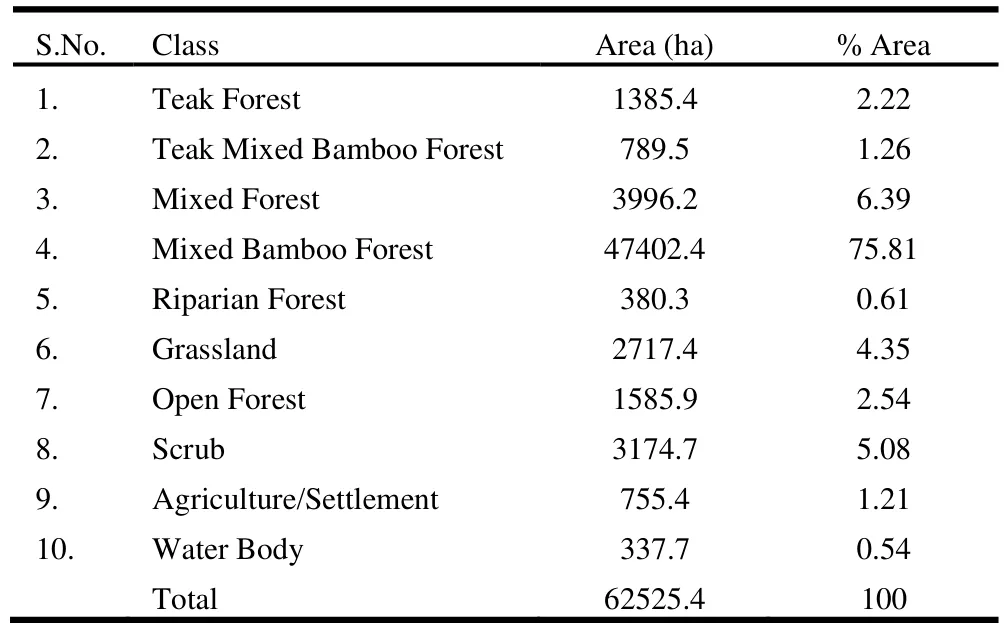
Table2. Area of landcover classes delineated

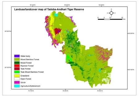
Fig.4. Landuse/landcover map of Tadoba-Andhari Tiger Reserve

Landscape pattern and structure

Landscapes in the study area had been defined at three levels of hierarchy starting from broader levels to narrower ones, i.e. landscape level, class level and patch level.

At Landscape Level

Tadoba-Andhari Tiger Reserve’s landscape was found to be heterogeneous in nature. As shown in Table3, a total of 2307 patches of different types and varying patch sizes (mean patch size =25.67 ha) could be recognized in the landscape with a patch density of 1.7 patch per km². The landscape was evenly interspersed with different forest types as indicated by the interspersion value of 50. The landscape was not very diverse in nature as shown by low values of Simpson Diversity index 0.38 and Simpson Evenness index 0.42.

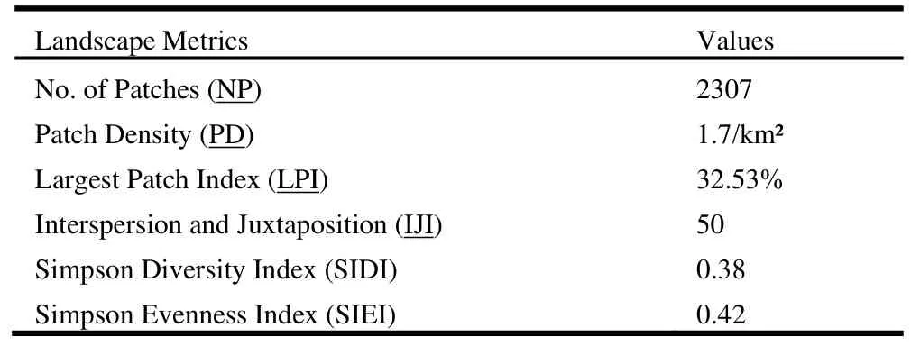
Table3. Landscape metrics for TATR landscape

At Class Level

The landscape was composed of six major vegetation types, viz.,mixed bamboo forest, mixed forest, teak forest, teak mixed bamboo forest, riparian forest and grassland have described. The result of all the metrics computed at the class level is given in Table4.

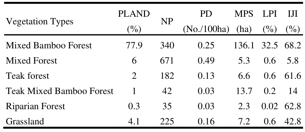
Table4. Class level metrics for landscape of TATR

Area and density metrics: Amongst all vegetation types,maximum percentage of land was covered by mixed bamboo forest (77.99%) with the highest mean patch size (136.09 ha) and the largest patch index (32.53%). Mixed forest has the highest number of patches (671) and therefore has the highest patch density (0.49/100ha). However, riparian forest had the least landscape area (0.3%) with lowest number of patches (35) and lowest mean patch size (2.25 ha). The average patch size varies from2.25 ha to 136 ha. Apart from mixed bamboo forest, all forest types have mean patch size below 15 ha.

Interspersion Metrics: The value of the interspersion / juxtaposition metric was found to be highest in mixed bamboo forest(75.23%) followed by riparian forest (62.79) and teak forest(61.63%). The least interspersion was found in mixed forest(5.78%).

At Patch level

The area of each patch comprising a landscape mosaic is the most useful piece of information contained in a landscape. The analyses revealed that among all the vegetation classes, mixed forest has the maximum number of patches among all vegetation classes. The small-size patches ranging from 0.5 to 5 ha were highest in number (599) and the large-size patches (above 100ha)were few. Among all vegetation classes in the TATR landscape,riparian forest had least number of patches (35) with 18 patches of size ranging from 0.5–5 ha and only one big patch of 22 ha.

Discussion

Vegetation Mapping

Landscape elements, coupled with satellite imagery can be effectively used to monitor biodiversity (Nagendra and Gadgil 1999).At high spatial resolution, many factors affect the recorded reflectance of the plant communities (species, crown closure,crown geometry, stand density, soil moisture and sun angle).This made it possible to map the communities. Despite using high-resolution satellite data, problems were encountered while mapping land-cover classes, since the presence of bamboo in the understory created a spectral overlap with spectral signatures of crown cover. Special consideration was given to the compatibility of collected ground data and the spectral qualities measured by satellite. Among the land-cover classes, mixed bamboo forest was the most dominant class in TATR because of extensive bamboo growth. Despite, teak being a dominant tree species in the study area, little area was occupied by pure teak patches. It is present only in the northern part of Tadoba National Park. Teak was mostly present along with its associates and bamboo in other forest types. The old plantations of teak have now been converted into teak mixed bamboo forest, because of extensive flowering of bamboo in TATR in the mid 1980s (Dubey and Mathur 1999). The scrub and open forest were mostly found in the southern part of the Andhari Wildlife Sanctuary. It could be attributed to villages present in the periphery of the southern zone, which exert an anthropogenic pressure that leads to the degradation of the surrounding forests. The presence of natural water sources and high protection status are major reasons contributing to the presence of all vegetation classes in Tadoba National Park.

Landscape Characterization

Structural analysis of the landscape helps in problem identification and the degree of severity, which is useful in ecosystem management (Formon and Godron 1986). The analysis here supports the observation that a small set of indices can capture significant aspects of landscape pattern. Structural analysis of the TATR landscape reveals its heterogeneous nature with large variations in patch size, but with low diversity, low evenness,and intermediate interspersion of forest types. Mixed bamboo forest covers the maximum area of TATR and therefore, the maximum percentage of the TATR landscape (77.99%), indicating its dominance among vegetation classes. Percentage landscape at the class level is a good indicator of fragmentation(Sinha and Sharma 2006). Mixed forest was found to be the most patchy, with the highest number of patches (671) and the highest patch density (0.49/100 ha). Our results have shown an interesting pattern, however: despite being dominant in the area, mixed bamboo forest has low patch density (0.25/100 ha). Despite having few patches, it had highest mean patch size (136 ha). Dominance of mixed bamboo forest is attributed to large-size patches,not to the number of patches.

Mixed bamboo forest and riparian forest had the highest adjacencies among all the vegetation types, indicating that these two forest types share their edges with the rest of the forest types.Nevertheless, teak mixed bamboo forest and mixed forest had the least interspersion among all forest types, due to their clumped distribution in the landscape.

This study has focussed on the approach of integrating satellite forest classification and forest inventory data for studying forest landscape patterns. IRS P6 LISS IV data have proved to have immense potential for minutely capturing the structural details of the landscape due to its high resolution and multispectral nature.This attribute has also been used for analyzing the patch dynamics in the landscape. The results presented here support focusing on a few metrics that represent overall landscape structure for landscape characterization and monitoring. Park managers should consider indices as tools for comparing different landscapes patterns. The trends depicted by the application of landscape metrics may be assimilated into their prognostic models and scenarios to support strategic decision making for regional conservation and policy development.

Conclusion

The TATR landscape is comprised of 10 landuse/landcover classes. Six major vegetation types—mixed bamboo forest,mixed forest, teak forest, teak mixed bamboo forest, riparian forest and grassland—were delineated. Mixed bamboo forest was the most dominant vegetation class, covering 75.81% of TATR,and riparian forest was the least represented, covering 0.61%.Detailed landscape-level analysis on the number of patches,patch characteristics (composition), spatial arrangement, and proximity of different patches (configuration) has provided crucial information on the landscape structure. Structural analysis of the TATR landscape revealed its heterogeneous nature with large variations in patch size. The landscape was found to have uneven distribution of the patches with intermediate interspersion among forest types. The dominance of mixed bamboo forest is attributedto the large size of the patches, despite being less in number.Mixed forest was found to have highest number of patches (671)and therefore the highest patch density (0.49/ha), while riparian forest has lowest patch density (0.03/ha). The results indicate that the landscape metrics in FRAGSTATS are effective in characterizing the landscape. This component of the our study has demonstrated the efficacy of high-resolution satellite IRS P6 LISS IV data with multispectral capability in detailed mapping of forest types with sharp boundaries and accurate area estimates.

Acknowledgements

We wish to thank the National Natural Resource Management System (NNRMS) and Ministry of Environment and Forests(MoEF), Government of India for funding the project “Mapping of National Parks and Wildlife Sanctuaries” from which the component of the study was extracted. We are also grateful to Maharashtra Forest Department and TATR management for support and cooperation in the field.

Bahuguna A. 2004. Evaluation of high resolution Resourcesat-1 LISSIV data for coastal zone studies. In: National Natural Remote Management System,NNRMS Bulletin. Hyderabad: National Remote Sensing Agency.

Champion HG, Seth SK. 2005. A Revised Survey of the Forest Types of India.Dehradun: Natraj Publishers.

Cherill AJ, McClean C. 1995. A comparison of land cover types in an Ecological field survey in northern England and a remotely sensed land cover map of Great Britain. Biological Conservation, 71: 313-323.

Chust G, Ducrot D, Pretus JL. 2004. Land cover mapping with patch-derived landscape indices. Landscape and Urban Planning, 69: 437-449.

Correy RC, Nassauer JI. 2005. Limitations of using landscape pattern indices to evaluate the ecological consequences of alternative plans and designs.Landscape and Urban Planning, 72: 265-280.

Cousins SAO, Eriksson O. 2002. The influence of management history and habitat on plant species richness in a rural hemi boreal landscape, Sweden.Landscape Ecology, 17: 517-529.

Cushman SA, McGarigal K, Neel MC. 2008. Parsimony in landscape metrics:Strength, universality, and consistency. Ecological Indicators, 8: 691-703.

Dubey Y, Mathur VB 1999. Establishing computerized wildlife database for conservation, monitoring and evaluation in Tadoba-Andhari Tiger Reserve,Maharashtra. Final project report. Wildlife Institute of India.

Dubey Y. 1999. Application of Geographic Information System in assessing habitat, resource availability and its management in Tadoba-Andhari Tiger Reserve. Ph.D Thesis submitted in Forest Research Institute (Deemed University) Dehradun. p. 250.

Formon RTT, Godron M. 1986. Landscape Ecology. New York, USA: John Wiley & Sons.

Franklin SE, Titus BD, Gillespie RT. 1994. Remote sensing of vegetation cover at forest regeneration site. Global Ecology and Biogeography Letters,4: 40-46.

Gachet S, Leduc A, Bergeron Y, Nguyen-Xuan T, Tremblay F. 2007. Understorey vegetation of boreal tree plantations: difference in relation to previous land use and natural forests. Forest Ecology and Management, 242:49-57.

Gould W. 2000. Remote sensing of vegetation, plant species richness and regional biodiversity hotspots. Ecological Applications, 10: 1861-1870.

Griffith JA, Martinko EA, Price KP. 2000. Landscape structure analysis of Kansas at three scales. Landscape and Urban Planning, 52: 45- 61.

Groom GB, Fuller RM, Jones AR. 1996. Contextual correction: techniques for improving land cover mapping from remotely sensed images. International Journal of Remote Sensing, 17: 69-89.

Gupta K, Jain S. 2005. Enhanced capabilities of IRS P6 LISS IV sensor for urban mapping. Current Science, 89: 1805-1812.

Innes JI, Koch B. 1998. Forest biodiversity and its assessment by remote sensing. Global Ecology and Biogeography Letters, 7: 397-419.

Jadhav RN, Murthy, AK, Chauhan KK, Tandon MN, Arravatia AML, Kandya K, Saratbabu G, Oza MP, Kimothi MM, Sharma K, Thesia JK. 1990. Manual of procedures for forest mapping and damage detection using satellite data, IRS-UP/ SAC/ FMDD/ TN/16/90.

Kulkarni AV, Bahuguna IM, Rathore BP, Singh SK, Randhwa SS, Sood RK,Dhar S. 2007. Glacial retreat in Himalaya using Indian remote sensing satellite data. Current Science, 92: 69-74.

Kumar V, Martha TR. 2004. Evaluation of Resourcesat-1 data for geological studies. In: National Natural Remote Management System, NNRMS Bulletin(B) 29, Hyderabad: National Remote Sensing Agency.

Lele N, Joshi PK, Agrawal SP. 2008. Assessing forest fragmentation in northeastern region (NER) of India using landscape matrices. Ecological Indicators, 8: 657-663.

Lilesand TM, Kiefer RW. 1994. Remote Sensing and image interpretation.New York.

Lu L, Li X, Cheng GD. 2003. Landscape evolution in the middle Heihe River Basin of north-west China during the last decade. Journal of Arid Environments. 53(3): 395-408.

McGarigal K, Marks BJ. 1995. FRAGSTATS: spatial pattern analysis program for quantifying landscape structure. Gen. Tech. Rep. PNW-GTR-351.Portland, OR: U.S. Department of Agriculture, Forest Service, Pacific Northwest Research Station, p.122.

Milanova EV, Lioubimtseva E Yu, Tcherkashin PA,Yanvareva LF. 1999.Land use/ Land cover change in Russia: mapping and GIS. Land use Policy,16(3): 153-159.

Miyamoto A, Sano M. 2008. The influence of forest management on landscape structure in the cool temperate forest region of central Japan. Landscape and Urban Planning, 86: 248-256.

Nagendra H, Gadgil M. 1999. Satellite imagery as a tool for monitoring species diversity: an assessment. Journal of Applied Ecology, 36: 388-397.

O’Neill RV, Krummel JR, Gardner RH, Jackson B, DeAngelis DL, Milne BT,Turner MG, Zygmunt B, Christensen SW, Dale VH, Graham RL. 1988. Indices of landscape pattern. Landscape Ecology, 1: 153-162.

Rajankar PB, Balamwar SV, Shrivastava NT, Sinha AK. 2004. Utilization of Resourcesat-1 data in agriculture applications. In: National Natural Remote Management System, NNRMS Bulletin. Hyderabad: National Remote Sensing Agency.

Rao KN, Narendra K. 2006. Mapping and evaluation of urban sprawling in the Mehasdrigedda watershed in Visakhapatnam metropolitan region using remote sensing and GIS. Current Science, 91: 1552-1557.

Sarangi RK, Chauhan P, Nayak S. 2004. Assessment of Resourcesat-1 AWiFS data for marine applications. In: National Natural Remote Management System, NNRMS Bulletin. Hyderabad: National Remote Sensing Agency.

Sharma A. 2009. Comparing the radiometric behavior of LISS III data of IRS1D and IRS P6 for landscape ccological application. Environmental Informatics, 13: 66-74.

Sinha R, Sharma A. 2006 Disturbance gradient analysis at landscape level in Daltonganj South Forest Division. Journal of Indian Society of Remote Sensing, 34: 233-243.

Skole D, Tucker C. 1993. Tropical deforestation and habitat fragmentation in the Amazon: satellite data from 1978 to 1988. Science, 26: 1905-1910.

Turner MG, Gardner RH, O’Neill RV. 2001. Landscape Ecology In Theory And Practice Pattern and Process. New York, USA Springer-Verlag,pp.1-23.

Turner MG. 1987. Landscape heterogeneity and disturbance. New York:Springer-Verlag.

Turner MG. 1990. Spatial and temporal analysis of landscape pattern, Landscape Ecology, 3: 153-162.

Wiens JA. 1995. Landscapes mosaic and ecological theory. In: L. Hansson, L.Fahrig, and G. Merriam (eds), Mosaics Landscapes and Ecological Processes. London, UK: Chapman & Hall, pp. 1-26.