Two Probability Plots of the Three-Parameter Lognormal Distribution

JIANG Ren-yan (蒋仁言)

College of Automotive and Mechanical Engineering, Changsha University of Science and Technology, Changsha 410114, China

Two Probability Plots of the Three-Parameter Lognormal Distribution

JIANG Ren-yan (蒋仁言)*

CollegeofAutomotiveandMechanicalEngineering,ChangshaUniversityofScienceandTechnology,Changsha410114,China

The two-parameter lognormal distribution is a variant of the normal distribution and the three-parameter lognormal distribution is an extension of the two-parameter lognormal distribution by introducing a location parameter. TheQ-Qplot of the three-parameter lognormal distribution is widely used. To obtain theQ-Qplot one needs to iteratively try different values of the shape parameter and subjectively judge the linearity of theQ-Qplot. In this paper, a mathematical method was proposed to determine the value of the shape parameter so as to simplify the generation of theQ-Qplot. Then a new probability plot was proposed, which was more easily obtained and provided more accurate parameter estimates than theQ-Qplot. These are illustrated by three real-world examples.

three-parameterlognormaldistribution;probabilityplot;correlationcoefficient;modelselection;parameterestimation

Introduction

The probability plot of a distribution model provides the information whether or not it is appropriate for fitting a given dataset[5]. When it is appropriate, one can obtain the parameter estimates from the data probability plot.

TheQ-Qplot of the three-parameter lognormal distribution has been widely used[1]. To obtain the lognormalQ-Qplot, one must first specify a value ofσl. This involves iteratively trying different values ofσland subjectively judging the linearity degree of the correspondingQ-Qplot. To improve this traditional approach, we present a mathematical method to determine the value ofσlin this paper. The proposed method is based on maximizing the probability plot correlation coefficient (PPCC)[6].

The paper is organized as follows. We first discuss theQ-Qplot in Section 1. The new probability plot is developed in Section 2. We compare their performances in Section 3. The paper is concluded in Section 4.

1 Lognormal Q-Q Plot

The two-parameter lognormal distribution is given by

(1)

where Φ[·] is the standard normal distribution. It is noted that the scale parameterμlis the logarithm of median life.

The three-parameter lognormal distribution is given by

(2)

The median life is given by

t0.5=eμl+γ.

(3)

Let

(4)

IfThas the cumulative distribution function (CDF) given by Eq. (2),Xfollows the two-parameter lognormal distribution with shape parameterσland scale parameterμl=0. Theα-fractile ofXis given by

xα=exp[Φ-1(α; 0,σl)],

(5)

where Φ-1(α; 0,σl) is theα-fractile of the normal variable lnX. From Eqs. (4) - (5), we have

tα=γ+eμlxα.

(6)

The plot oftαversusxαis a straight line, and we call it the lognormalQ-Qplot. Clearly, the lognormalQ-Qplot depends on the value ofσl. We propose an approach to specifyσlas follows.

Consider a complete dataset

t1≤t2≤…≤tn.

(7)

The empirical distribution function (or plotting position)Fiattiis given by[7]

Fi=betainv(0.5;i,n+1-i),

(8)

wherebetainv(0.5;a,b) is the median of the beta distribution defined in (0, 1) with shape parametersaandb, respectively. The methods to determine the plotting position for an incomplete dataset can be found from statistics or reliability related books[8].

Once the plotting position is determined, thexcoordinate of the point of theQ-Qplot associated withtican be calculated by Eq. (5) withα=Fi, and theycoordinate is given byyi=ti. For a given value ofσl, the PPCC is calculated as

ρ(σl)=correl(xi,yi; 1≤i≤n),

(9)

wherecorrel(X,Y) is the correlation coefficient betweenXandY. We determine the value ofσlby maximizing the PPCC. Onceσlis specified, we fit the data points of theQ-Qplot to the straight line equation given by

y=a0+a1x.

(10)

Comparing Eq. (10) with Eq. (6), we have

γ=a0,μl=lna1.

(11)

In such a way, all the parameters are estimated graphically.

2 Another Probability Plot of the Lognormal Distribution

Different from theQ-Qplot, we let

Y=ln(T-γ).

(12)

yα=μl+σlxα.

(13)

The plot ofyαversusxαis a straight line. SinceXandYhave the dimension of lnT, we call the new probability plot the lognormal lnQ-lnQplot.

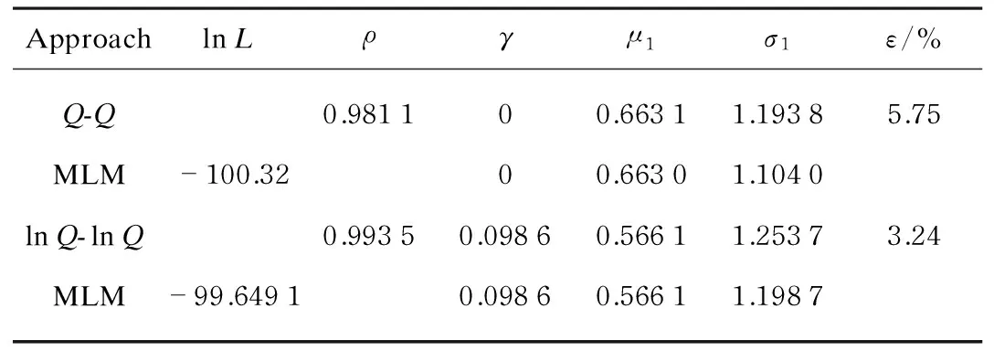
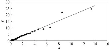
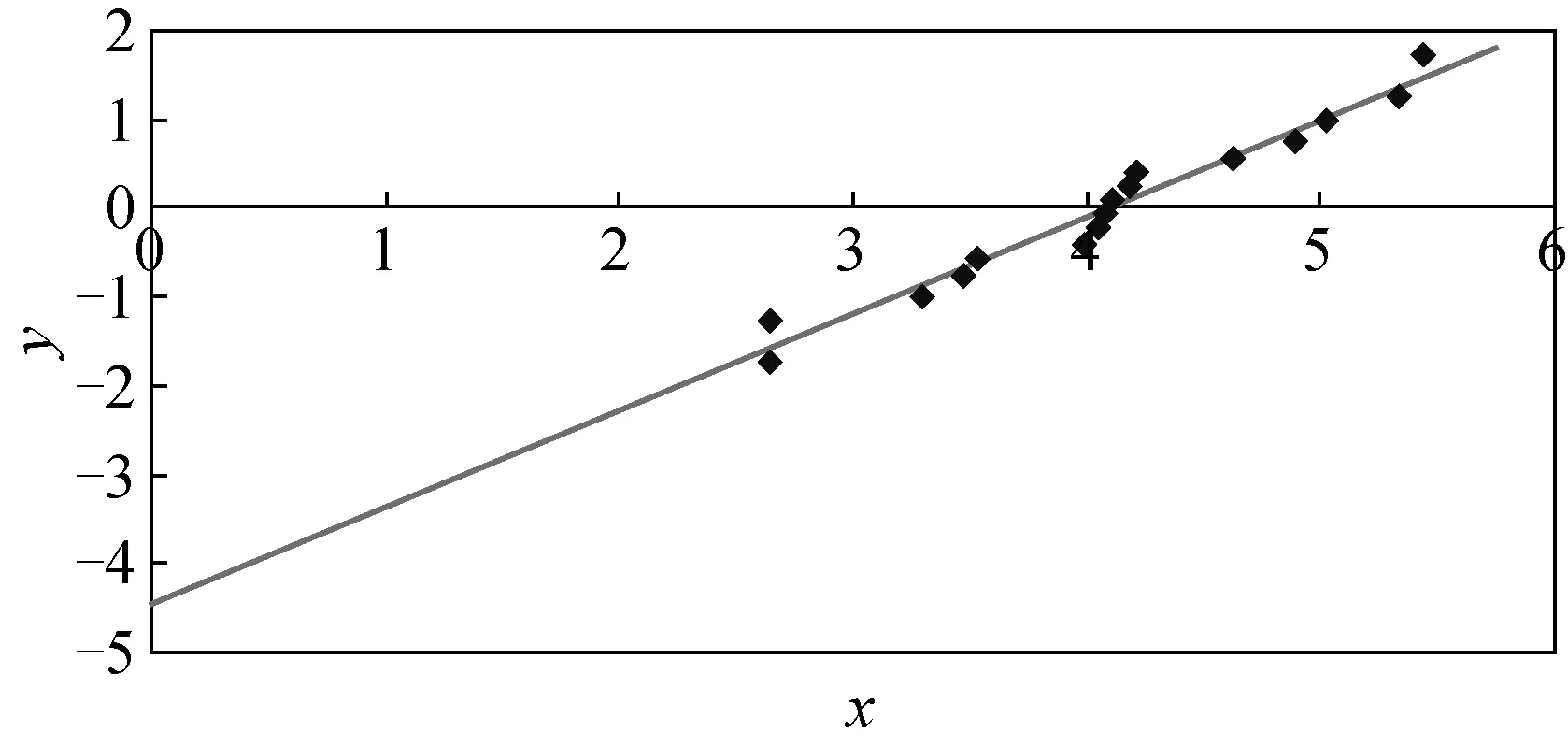
0≤γ

(14)

Clearly, it is much simpler to obtain the lnQ-lnQplot than to obtain theQ-Qplot. We show in the next section that the parameters estimated from the lnQ-lnQplot are more accurate than the ones estimated from theQ-Qplot.

3 Performances of Two Probability Plots

In this section we look at the performance of two probability plots by examining three real-world datasets. The datasets come from Ref. [9], and can be appropriately modeled by the inverse Gaussian distribution. We will examine whether these datasets can be appropriately modeled by the three-parameter lognormal distribution.

3.1 Datasets

The first dataset given in Table 1 deals with active repair time for an airborne transceiver; the second dataset shown in Table 2 deals with the millions of revolutions to failure of 23 ball bearings in a life test study; and the third dataset given in Table 3 deals with operating hours between successive failures of air-conditioning equipment in a Boeing 720 aircraft.

0.20.30.50.50.50.50.60.60.70.70.70.80.81.01.01.01.01.11.31.51.51.51.52.02.02.22.52.73.73.03.33.34.04.04.54.75.05.45.47.07.58.89.010.322.024.5

Table 1 Repair time for airborne transceivers/h

Table 2 Number of revolutions (in millions) to failure of ball bearings

Table 3 Intervals between failures of air-conditioning equipment/h

3.2 Parameters estimated from the probability plots

The accuracy of the graphical estimates can be measured by

(15)

where the superscript “G” indicates the graphical estimate and the superscript “M” indicates ML estimate. In terms ofε, the lnQ-lnQplot outperforms theQ-Qplot.

Table 4 Results for dataset 1

The Q-QplotandlnQ-lnQplot of the data are displayed in Figs.1 and 2, respectively. It is easier for one to give a judgment about the appropriateness of the lognormal model from the lnQ-lnQplot than from the Q-Qplot.

Fig.1 Q-Q plot for dataset 1

Fig.2 ln Q-ln Q plot for dataset 1

Table5showstheestimatedparameters.Thetwoprobabilityplots(showninFigs. 3and4)givetheestimateofγ=0, and show fair linearity. This implies that the lognormal distribution is appropriate for fitting this dataset. Once more, the lnQ-lnQplot has a smaller value ofεthan the Q-Qplot.

Table 5 Results for dataset 2

Fig.3 Q-Q plot for dataset 2

Fig.4 ln Q-ln Q plot for dataset 2

Table 6 shows the estimated parameters and, Figs. 5 and 6 display the two probability plots, which give the estimate ofγ=0. The Q-QplotdoesnotsupporttheuseofthelognormalmodelbutthelnQ-lnQplot shows a good linearity. Therefore, the lognormal distribution may or may not be appropriate for fitting the dataset.

Table 6 Results for dataset 3

Fig.5 Q-Q plot for dataset 3

Fig.6 ln Q-ln Q plot for dataset 3

It is noted that the lnQ-lnQplot gives better estimates in terms ofε.

3.3 Summary

Based on the above analyses, we can conclude as follows.

(1) The proposed probability plot can be conveniently generated and gives robust parameter estimates.

(2) TheQ-Qplot is sensitive to the variability of the data and tends to reject a model, while the lnQ-lnQplot tends to accept a model.

(3) It seems thatεnegatively correlates withρ.

(4) If we can determine a critical value for the PPCC, we can determine whether or not the lognormal distribution is appropriate for fitting the dataset in a quantitative way. We have completed such a study and the results will be reported elsewhere.

(5) When a candidate model is considered to be appropriate for fitting a given dataset, it does not imply that the candidate model is uniquely appropriate for fitting the data. In fact, we have known that the log-Weibull distribution (see Ref. [10]) provides better fits to all the three datasets considered in this paper than the lognormal distribution.

4 Conclusions

In this paper, we have presented a mathematical method to generate theQ-Qplot of the three-parameter lognormal distribution and developed a new probability plot. We have illustrated that the proposed probability plot can be conveniently generated and gives more accurate parameter estimates than the lognormalQ-Qplot.

An interesting finding is that all the three datasets that can be modeled by the inverse Gaussian distribution and can also be appropriately modeled by the lognormal distribution and the log-Weibull distribution. This implies that modeling for a given dataset should consider several candidate models.

[1] Li B Z, Yashchin E, Christiansen C,etal. Application of Three-Parameter Lognormal Distribution in EM Data Analysis [J].MicroelectronicsReliability, 2006, 46(12): 2049-2055.

[2] Chen C. Tests of Fit for the Three-Parameter Lognormal Distribution [J].ComputationalStatistics&DataAnalysis, 2006, 50(6): 1418-1440.

[3] Jiang R, Ji P, Xiao X. Aging Property of Unimodal Failure Rate Models [J].ReliabilityEngineering&SystemSafety, 2003, 79(1): 113-116.

[4] Nagatsuka H, Balakrishnan N. A Consistent Parameter Estimation in the Three-Parameter Lognormal Distribution [J].JournalofStatisticalPlanningandInference, 2012, 142(7): 2071-2086.

[5] Tang L C, Tan A P, Ong S H. Planning Accelerated Life Tests with Three Constant Stress Levels [J].Computers&IndustrialEngineering, 2002, 42(2/3/4): 439- 446.

[6] Heo J H, Kho Y W, Shin H,etal. Regression Equations of Probability Plot Correlation Coefficient Test Statistics from Several Probability Distributions [J].JournalofHydrology, 2008, 355(1/2/3/4): 1-15.

[7] Jiang R. A New Bathtub Curve Model with a Finite Support [J].ReliabilityEngineering&SystemSafety, 2013, 119: 44-51.

[8] Murthy D N P, Xie M, Jiang R. Weibull Models [M]. Hoboken: John Wiley & Sons, 2003.

[9] Henze N, Klar B. Goodness-of-Fit Tests for the Inverse Gaussian Distribution Based on the Empirical Laplace Transform [J].AnnalsoftheInstituteofStatisticalMathematics, 2002, 54(2): 425-444.

[10] Hasumi T, Akimoto T, Aizawa Y. The Weibull-Log Weibull Distribution for Interoccurrence Times of Earthquakes [J]PhysicaA:StatisticalMechanicsandItsApplications, 2009, 388(4): 491-498.

Foundation item: National Natural Science Foundation of China (No. 71371035)

1672-5220(2014)06-0757-03

Received date: 2014-08-08

* Correspondence should be addressed to JIANG Ren-yan, E-mail: jiang@csust.edu.cn

CLC number: TB114.3 Document code: A