Adaptive Non linear Model Predictive Control Using an On-line Support Vector Regression Updating Strategy☆

Ping Wang,Chaohe Yang,Xuemin Tian*,Dexian Huang3State Key Laboratory of Heavy Oil Processing,China University of Petroleum,Qingdao 266580,China

2College of In formation and Control Engineering,China University of Petroleum,Qingdao 266580,China

3Department of Automation,Tsinghua University,Beijing 100084,China

Adaptive Non linear Model Predictive Control Using an On-line Support Vector Regression Updating Strategy☆

Ping Wang1,2,Chaohe Yang1,Xuemin Tian2,*,Dexian Huang31State Key Laboratory of Heavy Oil Processing,China University of Petroleum,Qingdao 266580,China

2College of In formation and Control Engineering,China University of Petroleum,Qingdao 266580,China

3Department of Automation,Tsinghua University,Beijing 100084,China

A R T I c L E IN F o

Article history:

Received 24 June 2013

Received in revised form 14 October 2013 Accepted 16 November 2013

Available on line 20 June 2014

Adaptive control

Support vector regression

Updating strategy

Model predictive control

The performance of data-driven models relies heavily on the amount and quality of training samples,so it might deteriorate significantly in the regions where samples are scarce.The objective of this paper is to develop an online SVR model updating strategy to track the change in the process characteristics efficiently with affordable computational burden.This is achieved by adding a new sample that violates the Karush-Kuhn-Tucker conditions of the existing SVRmodeland by deleting the old sample that has the maximum distance with respect to the newly added sample in feature space.The benefits offered by such an updating strategy are exploited to develop an adaptive model-based control scheme,where model updating and control task perform alternately. The effectiveness of the adaptive controller is demonstrated by simulation study on a continuous stirred tank reactor.The results reveal that the adaptive MPC scheme outperform s its non-adaptive counterpart for large magnitude set point changes and variations in process parameters.

©2014 Chemical Industry and Engineering Society of China,and Chemical Industry Press.All rights reserved.

1.Introduction

Model predictive control(MPC)has been widely accepted as an advanced control strategy in process industry owing to its ability to handle complex control problems with constraints[1,2].MPC uses a process model to predict future process behavior and future control actions are computed by minimizing a pre-specified cost function,so the effectiveness of MPC relies heavily on the availability of a reasonably accurate process model.Until recently,industrial applications of MPC have mainly based on linear models due to their inherent simplicity from conceptual and implementation points of view[1].However,as many chemical plants exhibit highly nonlinear behavior when operated over a wide range,linear MPC often results in poor control performance, which motivates its extension to nonlinear MPC,with am ore accurate nonlinear model used for prediction and optimization[3].

Among various nonlinear modeling methods,the support vector regression(SVR)method has been widely applied in data-d riven modeling[4],since it not only shares many of its features with neural networks but also possesses some additional desirable characteristics. The advantage of SVR is that[4],for a given modeling problem with a finite set of samples,it can automatically derive the optimal network structure with respect to generalization error.Further more,current experience shows that SVRs work as well as,and in some cases,better than classical statistical approaches on noisy or imprecise data.Because of these advantages,SVR has been found increasing applications in chemical processes[5],especially when training data are in sufficient or the process has strong nonlinearity[6-8].Nevertheless,a basic limitation of all data-d riven models is their inability to extrapolate accurately once the in formation is outside the range of data used to generate the model[9].As the training samples available only describes a period of process historical behavior and might not represent complete characteristics of true dynamics,the performance of the model may deteriorate substantially with time as a consequence of changes in the dynamics of process[10-14].Although the model can be retrained from scratch when the training set is modified,it is cumbersome and computation ally inefficient.In this case,the accurate on line SVR (AOSVR)technique[15]seems to be a better alternative to SVR because it uses an incremental algorithm,which updates SVR model efficiently and accurately when a new sample is added to the training set without retraining from scratch.Several model-based control schemes based on AOSVR have been developed in recent years.Iplikci has proposed an adaptive generalized predictive control(GPC)method by combining SVR-based GPCapproach with AOSVR[16].An adaptive inverse control algorithm,where SVR model is used to construct the inverse model ofthe process to be controlled on line,has been studied[17].More recently,AOSVR is employed to capture the abrupt and incremental faults in the framework of SVR model based fault tolerance predictive control scheme[18].However,in these applications the AOSVR technique is used without taking in to account the differences among the newly incoming samples and lacking mechanisms to prune redundant samples efficiently[10].This may result in unreliable predictions and heavy computation burden as the number of training data increases,limiting the applications of recursive SVR algorithm to a long-term on line modeling and control task.

In our recent work,an efficient on-line model updating strategy based on AOSVR has been developed and shown good performance for predicting the melt index of an industrial polypropylene process [19].This strategy allows us to improve the estimation performance with affordable computation burden by updating the existing SVR model based on the novelty of new samples that arrive sequentially. In this paper,the benefits offered by such an updating strategy are further exploited to design an adaptive MPC controller.Several enhancements are also developed to make the model updating strategy capture the current behavior of process more effectively.Specifically, only those samples that violate the Karush-Kuhn-Tucker(KKT)conditions of existing SVR model are added to improve the estimation accuracy for new operating region where samples may not be scarce or nonexistent.As far as the accumulation of obsolete data is concerned, the old training sample with the maximum distance to the newly added sample in feature space will be recognized as the redundant sample,which will be removed from training database subsequently to enhance the estimation accuracy for the current behavior of process. The effectiveness of the adaptive MPC controller is illustrated by a simulation study on a benchmark continuous stirred tank reactor(CSTR) [20].The adaptive MPC controller is able to achieve a smooth transition for large magnitude set point changes and maintain the process at an unstable operating point in the presence of unmeasured disturbances and random noise.

2.On-line Support Vector Regression

Given a training set T={(χi,yi),i=1,2,…,N},where N is the total number of training samples,χi∈Rnis the n-dimension input vector,and yi∈R is the output variable.In the feature space F,SVR builds a linear regression function in the following form[4]

where w is a vector in F,Φ(⋅)is a mapping from the input space to the feature space,bis the bias term,and〈⋅,⋅〉stands for the inner product operation in F.The SVR algorithm s regard the regression problem as an optimization problem in dual space with the model given by

where ajis the coefficient of each sample and Kijdenotes the kernel function.Sample χjcorresponding to a non-zero ajvalue is referred to as the support vector(SV).By using Vapnik'sε-insensitive loss function, the dual form of the optimization problem becomes a quadratic programming(QP)problem

subject to constraints

where ε is the maximum value of tolerable error and C is a regularization parameter that represents a trade-off between model complexity and effect of tolerance to the error larger than ε.The Lagrange formulation of the QP problem can be further represented as

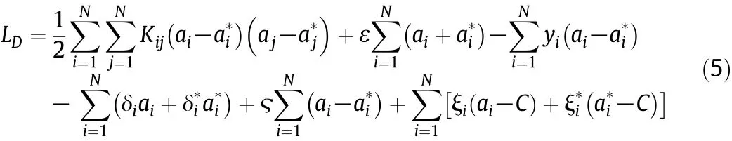
According to Eq.(6),at most one of aiandwill be nonzero and both are nonnegative.We define coefficient θiand margin function h(χi)as

Combining Eqs.(6)-(8),the KKT conditions can be rewritten as

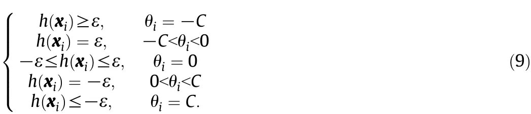
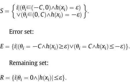
Based on Eq.(9),the training samples in T can be divided in to three subsets as follows[15].Support set:

The AOSVR algorithm consists of incremental algorithm and decremental algorithm[15].The basic idea of incremental algorithm is to find a way to add a new sample to one of the three sets maintaining KKT conditions consistent.When a new sample χcis received,its corresponding θcvalue is initially set to zero and then gradually changes under the KKT conditions.The relationship between h(χi),Δθiand Δb is given by

From Eq.(6),the relation bet ween θcand θiis

Among the three sets,only the support set samples can change θi, then the relation among Δθc,Δθjand Δ b can be formulated as[15]

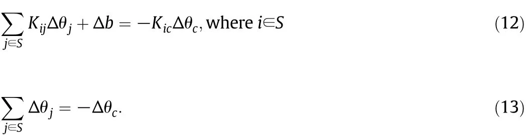
Defining the support set as a list of elem en ts S={s1,s2,…,sls}, Eqs.(12)and(13)can be rewritten in an equivalent matrix form

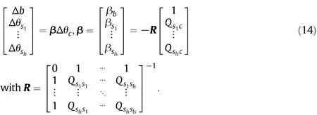
Updating θivalues,the support set samples will be consisten t. The h(χi)values for support samples do not need update,because they are always∣ε∣.For error and remaining samples,the situation is opposite.They do not change θivalue,but change h(χi).De fining N=E∪R=｛n1，n2，…，nln｝n ln and rewriting the variation of h(χi)in a matrix notation

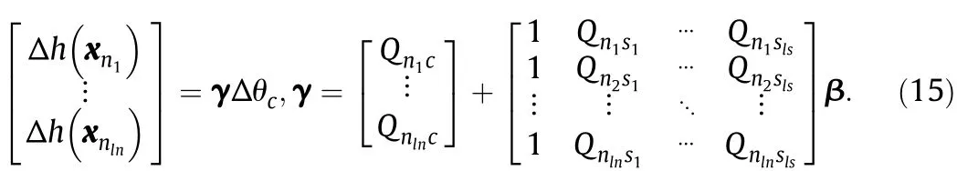
Δθi,Δb and h(χi)can be updated by computing β and γ.Eqs.(14) and(15)hold only when the samples in the support set do no t change membership.Therefore,Δ θcis chosen to be the largest value that can either maintain the support set unchanged or terminate the incremental algorithm.In this process,some samples may transfer from a set to another,and some may no t.The process is repeated until the KKT conditions are satisfied for all data points including the most recent one.Instead of solving a complex QP problem each time,the structure of SVR can ad just dynamically to meet the KKT conditions,making the AOSVR algorithm efficient for on line model updating[15-18].

3.Model Updating Strategy

3.1.Adding new samples based on KKT conditions

From a practical point of view,the idea of updating the existing model whenever a new sample is available is inappropriate,because frequently updating a model will result in high computation requirements and stability problems[11].More importantly,the generalization ability of the existing model may deteriorate significantly[10,19].An important prerequisite for successfully updating the existing model is that the newly added training samples contain enough new in formation.In this paper,the following proposition is used to distinguish the novelty of the training sample[19,21].

Proposition 1.Let f(χ)be the regression function of SV and{χc,yc}be a new sample.If{χc,yc}satisfies the KKT conditions,the SV set will not change,otherwise it will change.The samples that violate KKT conditions are those satisfying the following condition

Proposition 1 reveals the influence of a new sample on the SV set of the existing SVR model[21].If the new sample violates the KKT conditions,the SV set of SVR model will change after the incremental learning of the new sample.Since the training samples can be completely represented by the SV set,the KKT conditions seem to be more reasonable than regression functions in classifying the new samples and the SVR model should be updated according to the novelty of training data. When a new sample is added to the training set,the geometrical interpretation of the shift in the regression curve is illustrated in Fig.1. After adding new sample{χc,yc},the updated regression curve,denoted by f（χ）,is dragged towards the newly added sample in the high dimension feature space.In this way,the updated SVR model is able to absorb the in formation contained in the newly added sample.By introducing new samples selectively,the frequent update of the existing SVR model is avoided.Accordingly,the generalization ability of the model is well maintained,while the computation burden is reduced.

In applications,the outputs of process are always corrupted by random noise,leading to frequent model updating.To cope with this problem,a simple linear filter is introduced to smooth the training samples as it can be easily implemented on line.The process output is smoothed by a weighted sum of previous measurements in a window of finite length

where N0is the filter length,which can be ad justed according to the level of process noise,aiare filter coefficients with values between 0 and 1,and y（k）is the de-noised output.

3.2.Pruning old samples based on distance

The dimension of matrixes in Eqs.(14)and(15)increases with the accumulation of training samples,leading to excessive computation for model updating,especially when the model is used for control purpose[11,22].In addition,the updated model may fail to track changes in the process timely as the training set contains too many out-of-data samples.Considering all these factors,it is necessary to delete those samples as long as they become redundant.One of the simplest pruning strategies is to remove the oldest sample from the memory whenever a new one is added,assuming that the oldest sample is the one with the least contribution to the construction of existing model.However,inmany applications there is no guarantee that the oldest sample no longer represents the current behavior of process.Another common approach is to delete those samples that are not belonging to SVs,because SVR can be completely represented by the SV s.However,as mentioned earlier,samples may transfer from a non-SV to a SV during the implementation of AOSVR.Other pruning strategies,such as Bayesian and leave-one-out cross-validation,are mainly used in an offline manner because of their complexity[10].

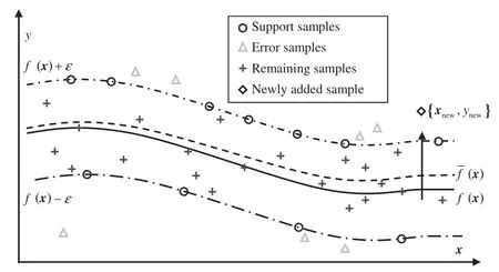
Fig.1.Geometrical interpretation of the shift in regression curve with a new sample added.

Discarding a training sample from the model might inevitably degrade its performance.Pruning rules aim at finding samples whose removal is expected to have negligible effect on the quality of the model.Fora new sample{χc,yc}added to the training set and the correspondingly updated SVR model f（χ）,the condition to confirm if some old training samples need to be deleted is

where ecis the approximation error of the updated SVR model with respect to the newly added sample and e1is a given threshold associated with model accuracy.If condition(18)is satisfied,the newly added sample is not yet adequately represented by the updated SVR model, and some old training samples should be deleted to enhance the estimation accuracy of the SVR model for the current behavior of process.Instead of pruning the oldest training sample,sample will be deleted according to its distance to the newly added sample in feature space. In feature space,the distance between sample χiand χcis defined as

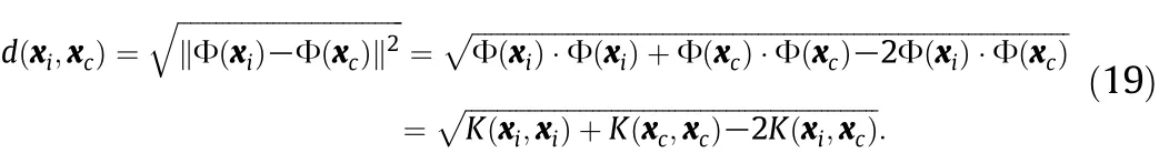
In the calculation of the distance in feature space,it does not need to know the explicit mapping function since it can be written solely in terms of the kernel function by the“kernel trick”.If condition(18)is satisfied or the number of training samples exceeds a given maximum limit,the sample with the maximum distance to the newly added sample will be removed from the training database in AOSVR.

When an old sample{χd,yd}is deleted,the geometrical interpretation of the shift in the updated SVR regression curve is illustrated in Fig.2.The regression curve of the updated model,denoted by f（χ）, tends to be d ragged towards the location of the newly added sample {χc,yc}after deleting the old sample.Considering that the kernel function of SVR is local in nature[23],it is anticipated that the estimation accuracy of the updated SVR model for the current behavior of process is improved.The relationship between the distribution of training samples and the robustness of SVR to outliers has been analyzed in detail[23].It is found that the influence of outliers on SVR depends on the distance between outliers and the SV s nearest to them.Therefore,even if an outlier enters the training set,it may not have significant impact on the model performance,since the outlier generally locates far away from those normal training samples.As long as the new correct samples are constantly fed to the training set,the outlier will be removed from the training set in time and,accordingly,the model may recover from its damage quickly.The robustness to outliers can be improved, in such a way,to avoid data in abnormal conditions distorting the model.The computation burden of the pruning strategy depends on the calculation of Eq.(19),which is relatively small and suitable for on line application.

The flowchart of the proposed model updating strategy is shown in Fig.3.When a sample is available,the KKT conditions will be checked according to Eq.(16).If this condition is satisfied,the existing model is considered accurate enough and does not need update.Otherwise,the new sample should be added to update the SVR model.After that,the accuracy of the updated model with respect to the newly added sample will be evaluated under the condition of Eq.(18).If it is satisfied or the sample number reaches the given limit,the distance bet ween the newly added sample and the old training samples is computed according to Eq.(19).The old sample with the largest distance is removed from the training set using the decremental algorithm.As a result,the updated model ad justs its structure to capture the changes in the process adaptively,while its size is maintained within a reasonable range with limited computation cost.

4.Non linear Model Predictive Con tro l

We assume that the process to be controlled can be described by the SVR model with the following structure[22,24]

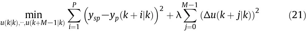
where y(k)and u(k)are the process output and input variables with lags nyand nu,respectively,e(t)is a white noise,and f(⋅)denotes the SVR model.At sampling instant k,the MPC problem is defined asa constrained optimization problem,where the future manipulated input moves are determined by minimizing the objective function

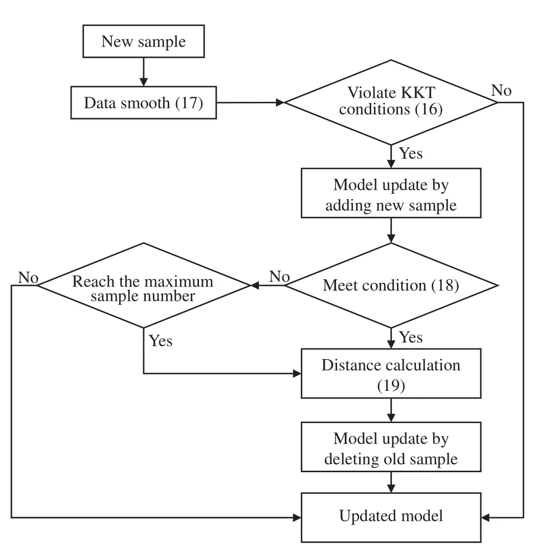
Fig.3.Flow chart of the model updating strategy.

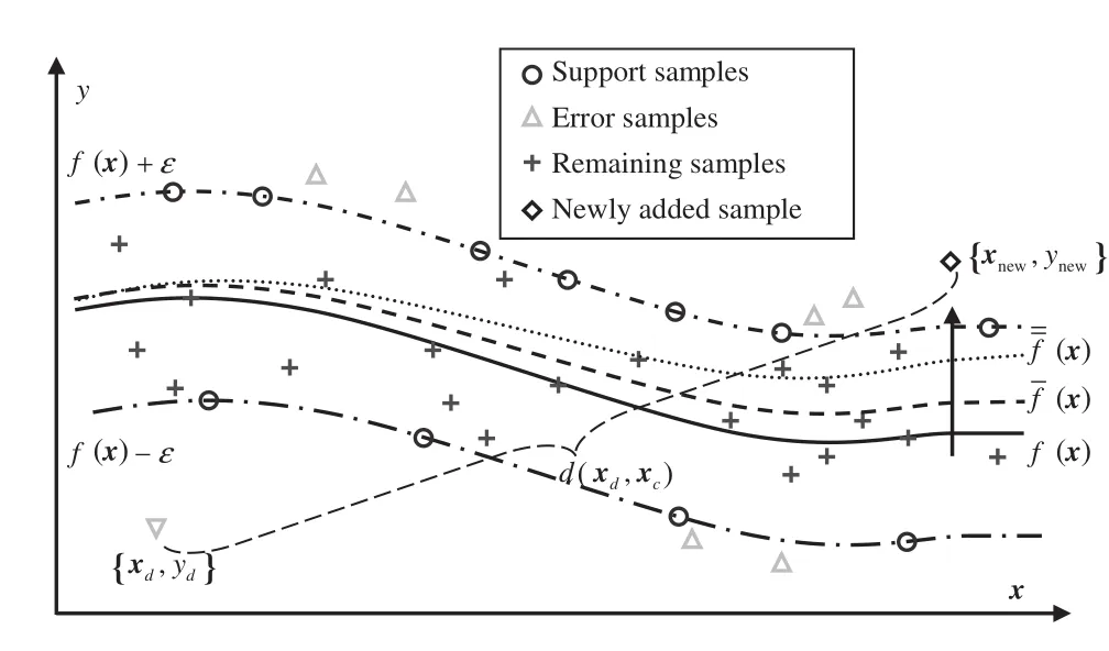
Fig.2.Geometrical interpretation of the shift in the regression curve with an old sample deleted.

subject to following constraints

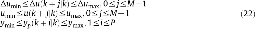
where yspis the set point of controlled variable,yp(k+i|k)denotes the model prediction for process output y(k+i)based on available measurements at sampling instant k,λ≥0 is a weighting factor,P and Mde note the prediction horizon and control horizon,respectively, Δu(k+j|k)is the future control increment,while u(k+j|k)denotes the control action at the future sampling instant k+j based on available measurements at instant k.The resulting constrained nonlinear optimization problem can be solved using standard nonlinear programming algorithms.MPC is implemented in a moving horizon manner,so after solving the optimization problem,only the first control action is applied to the plant and the optimization problem is reformulated at the next sampling instant k+1,based on the available in formation from the process.

The performance of MPC relies heavily on the quality of process model.However,even if an accurate model for the process is initially available,its performance may deteriorate substantially with time due to the shift at the operating point,changes in the disturbance characteristics,etc.Although the feedback mechanism of MPC tolerates some model mis matches,the presence of large plant-model mis match may deteriorate the control performance significantly.To cope with this problem,an adaptive nonlinear MPC algorithm based on the SVR model updating strategy is presented.Specifically,at sampling instant k,the accuracy of existing SVR model,denoted as fk(⋅),with respect to the new sample will bee valuated before it is used to provide predictions at sampling instant k+1.If it is not accurate enough to rep resent the process dynamics at the current operating point,it will be updated with the newly incoming sample,and control actions based on the current model will be applied to the process.Thus the adaptive control algorithm consists of two sub-stages,the model updating stage,where the model is updated to trace changes in the process and account for the modeling errors explicitly,and the control stage,where a nonlinear optimization problem is solved to yield control sequence and new samples for model updating.

5.Illustrative Example

An exothermic CSTR with irreversible reaction A→B is adopted to illustrate the method developed.The dynamic behavior of the CSTR process is described in a dimensionless form[20]

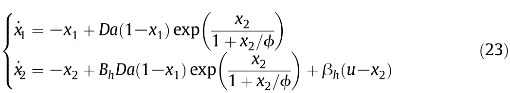
where χ1and χ2are the reactant concentration and temperature, respectively,u is the input of cooling jacket with constraints∣u∣≤2 and∣u∣≤0.25,Da is the Damkohler number,ϕ is the activation energy, Bhis the heat of reaction,and βhis the heat transfer coefficient.For Da=0.072,ϕ=20.0,Bh=8.0 and βh=0.3,the process exhibits output multiplicity and is open-loop unstable in the desired operating region[25].Three operating points are selected as the set points for simulations:A(χ1=0.144,χ2=0.8860,u=0.0)and C(χ1=0.7646,χ2= 4.7505,u=0.0)are stable operating points,and B(χ1=0.4472,χ2= 2.7517,u=0.0)is an unstable operating point.In this study,the output is y=χ1and the dimension less sample period is set to 0.5.

Initially,the SVR model is identified using the input-output data obtained from the closed-loop operation of the CSTR with a PID controller. The input and output lags are both set to 2.The parameters of the SVR model with the Gaussian kernel function are chosen as ε=0.01,C= 100 and σ=0.1.A set of 100 training data are used to train an initial SVR model,resulting in a model with 24 support vectors.For MPC,the prediction and control horizon are set to 7 and 2 samples,respectively, using different values and comparing control performance.The weighting factor λis set to 0.4.The measure men ts of the process output,χ1,are corrupted by the zero mean Gaussian white noise signals with the standard deviation of 0.05.It should be noted that identical parameters are chosen for all the MPC controllers in this section.Consequently,the conclusions drawn below do not depend on a particular choice of parameters. As far as the on-line model updating stage is concerned,the linear filter length N0is set to 6 and the threshold e1is set to 0.01.

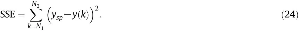
The performance of MPC controllers with adaptive(denoted as MPC1)and non-adaptive SVR models(denoted as MPC2)for set point tracking is first investigated.The simulation results are shown in Fig.4.The performance of the non-adaptive MPC controller is relatively good at the beginning,but deteriorates substantially with time as a consequence of shifts in the operating region.Specifically,when the set point changes from B to A at sample time 50 and changes from A back to B at sample time 100,the response of controller results in obvious steady state offset error and exhibits large overshoot behavior.The poor performance can be attributed to the lack of training data over the open-loop unstable region for the off-line trained model.In addition, it is noted that the output response for transition A to B shows an obvious spike,while the response for transition B to A is relatively smooth. This phenomenon is mainly caused by that B is an open-loop unstable operating point,which is more difficult to be controlled,compared with the stable operating point A.In contrast,the controller with adaptive model per forms well consistently over the operating range of interest,though the transitions among different operating points could excite inherent nonlinearity of the process and pose significant challenges for process control.It indicates that the inclusion of the model updating stage is able to cope with the problem of plant-model mismatches in different operating regions.

Fig.5 gives a better insight in to the effectiveness of the model updating strategy,where the change in the number of SVs is depicted. The SVR model is not updated frequently even the process is subjected to changes in the operating region and random noise.Specifically,only 13 new samples are added and 12 old samples are deleted,about 3% of all of the samples(400).Th is is different from the conventional AOSVR algorithm based adaptive controller,where all of the samples are used to update the SVR model,resulting in frequent changes in the model formulation and,thus,a large computation load for on line application.

The sum of squared error(SSE)between the set point and the process output over the sampling interval[N1,N2]is used to assess the control performance,defined as

The SSE values of the two controllers for set point tracking are listed in Table 1.The average CPU seconds needed by the two controllers at each step is also summarized in Table 1.The adaptive MPC controller outperforms the MPC based on the offline trained model,particularly when the process goes through the open-loop unstable region.It is noted that two controllers have nearly identical computation burden, though the adaptive controller needs to update the model whenever required.Com pared with the computation time needed for solving thenonlinear optimization problem,the time required by the model updating stage is rather limited.

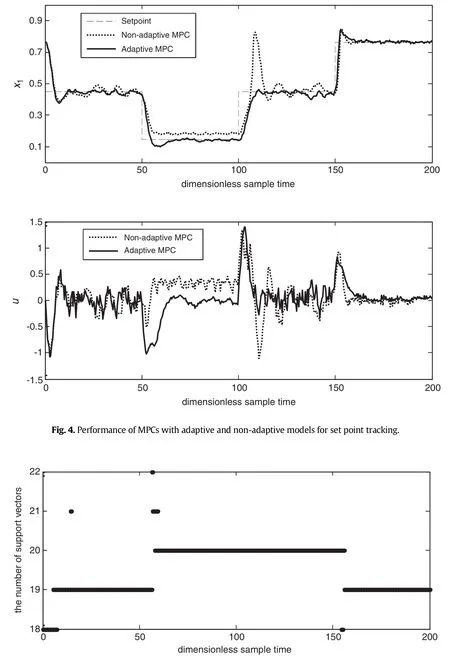
Fig.5.Changes in the number of support vectors of the updated SVR model.

Starting from the unstable operating point B,the activation energy ϕ increases to 110%of its nominal value at sample time 40 and then the heat transfer coefficient βhis subjected to a ramp type change withdecline rate of 5×10−3per sample time at sample time 100 until it reaches 88%of its nominal value at sample time 125.In this case,the task of controller is to maintain the process output at the unstable operating point B despite disturbances.Responses of the two controllers for disturbance rejection are depicted in Fig.6.The adaptive controller, which is able to recover from disturbances relatively quickly and maintain the process around the unstable operating point,showing better performance compared to its non-adaptive counterpart.

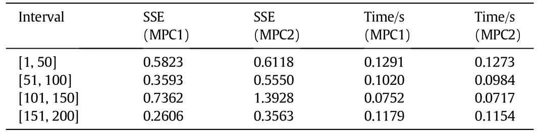
Table 1Performance of the two controllers for the set point tracking problem

In Table 2,the SSE values and computation time are presented for the two MPC controllers.The results confirm that the adaptive controller presents better performance than the non-adaptive one,with limited computation time in the model updating stage.For this application, we conclude that the proposed model updating strategy is able to provide necessary process representation for developing an efficient adaptive MPC scheme,for both set point tracking and disturbance rejection.

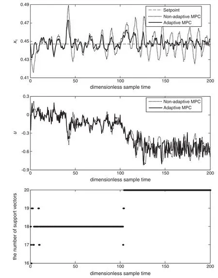
Fig.6.Performance of MPCs with adaptive and non-adaptive models for disturbance rejection.

6.Conclusions

Ame tho do logy for efficiently updating SVR models based on the AOSVR algorithm was proposed.This is achieved by adding new sample that violates the KKT conditions of the existing SVR model and deleting old samples that has the maximum distance with respect to the newly added sample in feature space.The advantage of the proposed method is that it offers a scheme to update the existing SVR model in an on line fashion with emphasizing the estimation accuracy for the current operating region.This provides a useful too l not only for predicting the behavior of time varying processes,but also for developing adaptive model-based control schemes.The effectiveness of the adaptive control scheme is illustrated in the simulation study for control of a CSTR process.The simulation results confirm that the adaptive controller could provide better control performance than the non-adaptive one,while the computation time required by the model updating stage is rather limited.Further work is in progress to incorporate some persistent excitation conditions in to the adaptive MPC scheme,according to process identification needs of the closed loop.

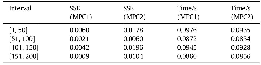
Table 2Perform ance of the two MPC controllers for disturbance rejection

[1]S.J.Qin,T.A.Badg well,A survey of industrial model predictive control technology, Control.Eng.Pract.11(7)(2003)733-764.

[2]S.Engell,Feedback control for optimal process operation,J.Process Control17(3) (2007)203-219.

[3]L.Magni,M.D.Raimondo,F.Allgower,Non linear model predictive control:tow ards new challenging applications,Lecture Notes in Control and In formation Sciences, vol.384,Springer-Verlag,Berlin,2009.

[4]J.A.K.Suykens,Support vector machines and kernel-based learning for dynamical systems modelling,Proceedings of the15th IFACSymposium on System Identification, Saint-Malo,France,2009,pp.1029-1037.

[5]S.B.Chitralekha,S.L.Shah,Application of support vector regression for developing soft sensors for nonlinear processes,Can.J.Chem.Eng.88(5)(2010)696-709.

[6]J.L.Wang,T.Yu,C.Y.Jin,On-line estimation of biomass in fermentation process using support vector machine,Chin.J.Chem.Eng.14(3)(2006)383-388.

[7]S.N.Zhang,F.L.Wang,D.K.He,R.D.Jia,Real-time product quality control for batch processes based on stacked least-squares support vector regression models,Com put. Chem.Eng.36(10)(2012)217-226.

[8]J.A.Yu,Bayesian inference based two-stage support vector regression framework for soft sensor development in batch bioprocesses,Com put.Chem.Eng.41(11)(2012) 134-144.

[9]P.Kad lec,R.Grbic,B.Gabrys,Review of adaptation mechanism s for data-driven soft sensors,Com put.Chem.Eng.35(1)(2011)1-24.

[10]J.l.Liu,Development of self-validating soft sensors using fast moving window partial least squares,Ind.Eng.Chem.Res.49(22)(2010)11530-11546.

[11]Y.Liu,H.Q.Wang,J.Yu,Selective recursive kernel learning for online identification of nonlinear systems with NARX form,J.Process Control20(2)(2010)181-194.

[12]L.J.Li,H.Y.Su,J.Chu,Modeling of isomerization of C8 aromatics by on line least squares support vector machine,Chin.J.Chem.Eng.17(3)(2009)437-444.

[13]K.Chen,J.Ji,H.Q.Wang,Adaptive localkernel-based learning for soft sensor modeling of nonlinear processes,Chem.Eng.Res.Des.89(10)(2011)2117-2124.

[14]D.Li,H.Li,T.Si,On-line robust modeling of nonlinear systems using support vector regression,Proceedings of 2nd International Conference on Advanced Computer Control(ICACC),Shenyang,China,2010,pp.204-208.

[15]J.Ma,J.Theiler,S.Perkins,Accurate on line support vector regression,NeuralCom put. 15(11)(2003)2683-2704.

[16]S.Iplikci,Online trained support vector machines-based generalized predictive control of non-linear systems,Int.J.Adapt.Control Sig.Process 20(10)(2006)599-621.

[17]H.Wang,D.Y.Pi,Y.X.Su,On line SVM regression algorithm-based adaptive inverse control,Neurocomputing 70(4-6)(2007)952-959.

[18]S.R.Sergio,M.J.Fuente,Fault tolerance in the framework of support vector machines based model predictive control,Eng.Appl.Artif.Intell.23(7)(2010)1127-1139.

[19]P.Wang,H.G.Tian,X.M.Tian,D.X.Huang,A new approach for on line adaptive modeling using incremental support vector regression,CIESC J.61(8)(2010) 2040-2045.

[20]J.Zhan,M.Ishida,The multi-step predictive control of nonlinear SISO processes with a neuralmodel predictive control(NMPC)method,Com put.Chem.Eng.21(2) (1997)201-210.

[21]W.D.Zhou,L.Zhang,L.C.Jiao,An analysis of SVMs generalization performance,Acta Electron.Sin.29(5)(2001)590-594.

[22]Y.Liu,Y.C.Gao,Z.L.Gao,H.Q.Wang,P.Li,Simple nonlinear predictive control strategy for chemical processes using sparse kernel learning with polynomial form,Ind.Eng. Chem.Res.49(17)(2010)8209-8218.

[23]E.Wael,K.Meh med,Local properties of RBF-SVM during training for incremental learning,Proceedings of International Joint Conference on Neural Networks,Atlanta, Georgia,USA,2009,pp.779-786.

[24]W.M.Zhang,G.L.He,D.Y.Pi,Y.X.Su,SVM with polynomial kernel function based nonlinear model one-step-ahead predictive control,Chin.J.Chem.Eng.13(3) (2005)373-379.

[25]E.Hernandez,Y.Arkun,Study of the control-relevant properties of back propagation neuralnet work models of nonlinear dynamical systems,Com put.Chem.Eng.16(4) (1992)227-240.

☆Supported by the National Basic Research Program of China(2012CB720500), Postdoctoral Science Foundation of China(2013M541964)and Fundamental Research Funds for the Central Universities(13CX05021A).

*Corresponding author.

E-mailaddress:tianxm@upc.edu.cn(X.Tian).