Global Existence and Pointwise Estimates of Solutions to Generalized Benjamin-Bona-Mahony Equations in Multi Dimensions∗

Hongmei XU Yan LIANG

1 Introduction

In this paper,we are interested in the global existence and time-asymptotic behavior of solutions to generalized Benjamin-Bona-Mahony(GBBM)equations in all space dimensions.The GBBM equation is defined as

whereu∈R1,ηis a positive constant,andβis a real constant vector.f(u)=(f1(u),···,fn(u))T,andfi(u)=u2,wherenis the space dimension.In this paper,n≥1.The initial data is given by

The well-known Benjamin-Bona-Mahony(BBM)equation is of the form

It was proposed and studied in[1]by Benjamin,Bona and Mahony for the special physical situations in the long wave limit for nonlinear dispersive media.Since then,the existence and uniqueness of solutions to various generalized BBM equaitons have been proved by many authors(see[1–4]).The decays of solutions were also studied in[5–9].However,most of these studies are in low space dimensions and the decay estimates are inLpnorm.The aim of this paper is to give the global existence and pointwise decay rates of solutions to Cauchy problems of the GBBM equation in all space dimensions.

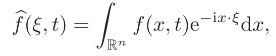
First we introduce some notations.As usual,Fourier transformation to the variablex∈Rnis

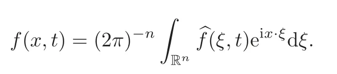
and the inverse Fourier transformation to the variableξis

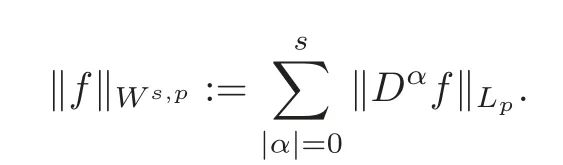
We also useF−1()to denote the inverse Fourier transformation of functionDαf=for multi-indexα=s∈Z+,p∈[1,∞],denotes the usual Sobelev space with the norm

In particular,We denote the generic constant byC.All the convolutions are about the spatial variablexin this paper.

We arrange this paper as follows.In Section 2,we derive the solution formula of the Cauchy problem.We need many inequalities in our analysis.We list the inequalities and their proofs in Section 3.We construct a solution sequence due to the solution formula of(1.1)–(1.2),and then prove that the sequence is a Cauchy sequence in a Banach space.Thus it converges to the solution of our problem.We leave these treatment processes to Section 4 and Section 5.Finally,we give our conclusion in Section 6.

2 Solution Formula

The aim of this section is to derive the solution formula from the problem(1.1)–(1.2).The linearized form of(1.1)is

Taking Fourier transform to variablexof(2.1),we have

The corresponding initial data is given by

The solution to the problem(2.2)–(2.3)is given by

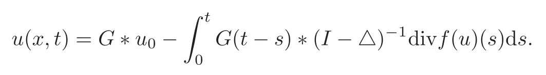
Set(ξ,t)=By the Duhamel principle,we get the solution formula for(1.1)–(1.2):

Set(ξ,t)=Then

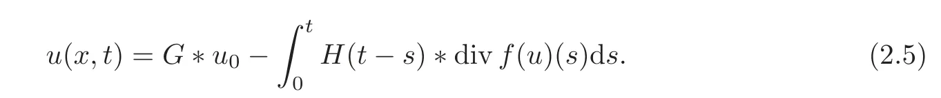
Due to(2.5),we define a solution sequencesatisfying

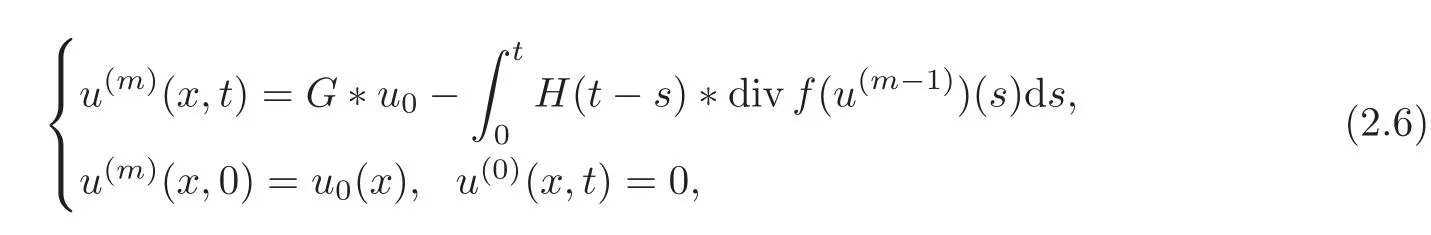
wherem≥1.Next we will prove thatis a Cauchy sequence in a Banach space,and then it converges to the solution to(1.1)–(1.2).To do so,we shall need many inequalities.We collect them in the following section.

3 Preliminaries

In order to estimatewe must analyse the decay property forG,Hfirst.Set

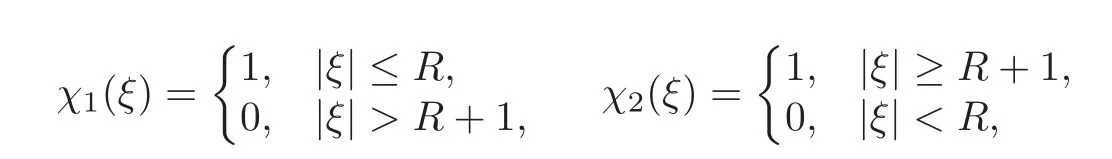
whereχ1,χ2are smooth cut-off functions andχ1(ξ)+χ2(ξ)=1.

Setfori=1,2.

ForG1,H1,we have the decay property as follows.

Lemma 3.1There exists a constantdepending on N,αsuch that

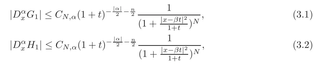
where N is a positive integer.Throughout this paper N＞

Conveniently,we next denoteBN(x,t)=

ProofWhen|ξ|is bounded,using the Taylor expansion,we have

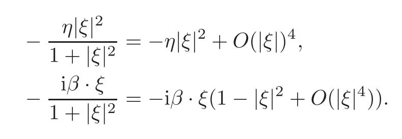
Then

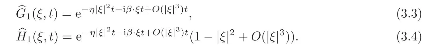
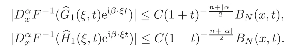
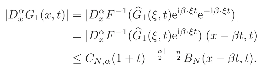
We know thatis a parallel operator.It can not contribute to the decay factor,but it has a physical meaning.So next we will not neglect the effect of the operator.From(3.3)–(3.4),we get

where(|α|−|β|)+:=

Then

Similarly we get(3.2).

G2,H2have the construction as follows.

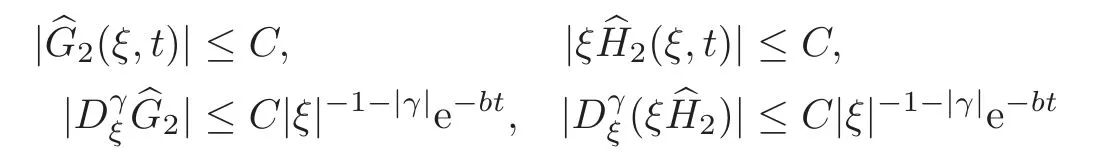
Lemma 3.2There exists a positive constant b and distributionsfor i=1,2such that

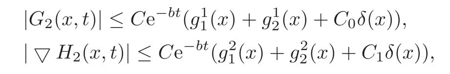
where δ(x)is Dirac function and

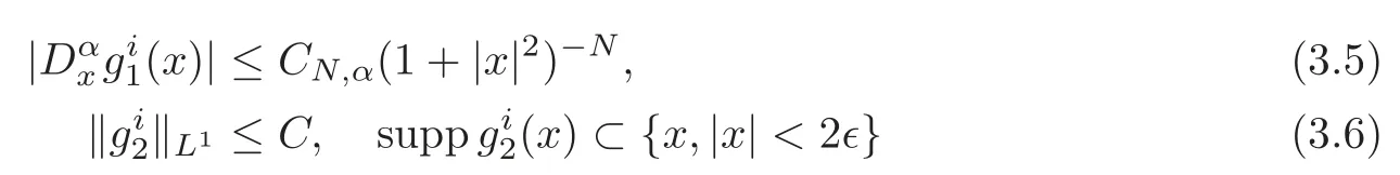
withbeing sufficiently small.

ProofWhen|ξ|is large enough,using Taylor expansions,we have

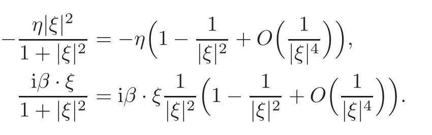
Thus we have

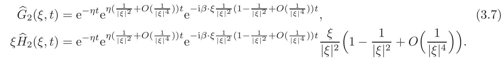
Then there exists a positive constantbsuch that

with|γ|≥1.From[10,Lemma 3.2],we get our results.

When dealing with the convolution with the nonlinearized part,we need the following four lemmas.

Lemma 3.3For positive constants b,N,when t is large enough,we have

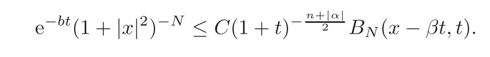
ProofNoticing thatifN,tare large enough,we have

Thus we get our lemma.

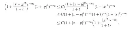
Lemma 3.4Whenand n3=min{n1,n2},we have

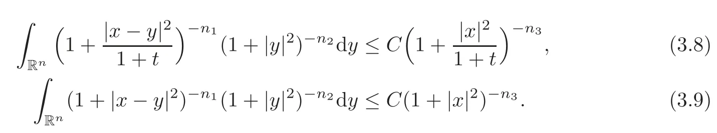
ProofWe just prove(3.8).The proof of(3.9)is similar.

When|x−y|(3.8)is easily got.

When|x−y|we have|y|Thus

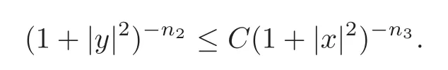
If|x|≤we haveBn3(x,t)≥C.(3.8)is easily got.

If|x|＞we have

Thus

Then(3.8)is proved.

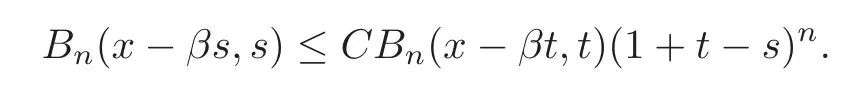
Set

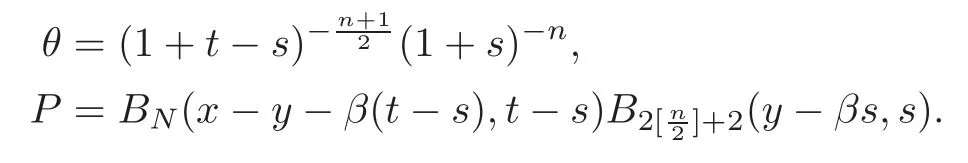
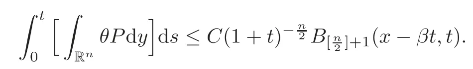
Lemma 3.5

ProofWe divide the proof into two different cases.

Case 1|x−

In this case,(x−βt,t)≥C.From[11,Lemma 5.2],we have

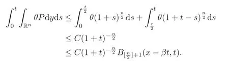
Case 2|x−βt|≥

We also divide the proof into two different cases.

Case 2.1s

If|y−βs|then

From[11,Lemma 5.2],we have

If|y−βs|≤then|x−y−β(t−s)|≥We have

Case 2.2s≥.

The proof of this part is similar to that of Case 2.1,so we omit it here.

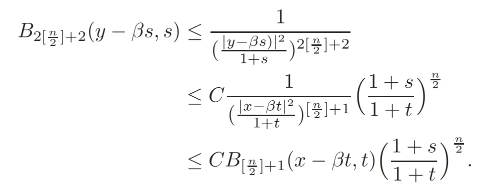
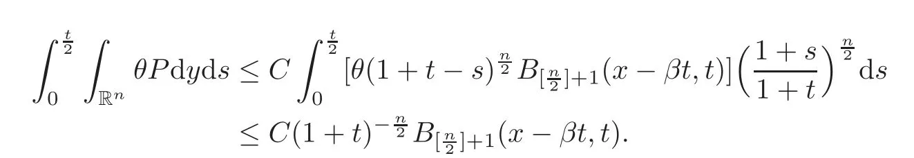
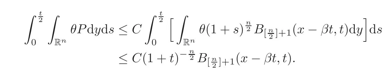
Lemma 3.6There exists a constant depending only on n such that

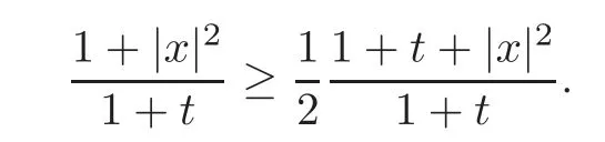
ProofSince|x−βt|2≤2(|x−βs|2+|β|2(t−s)2),we have

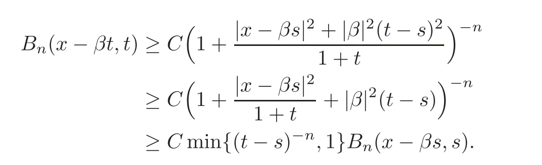
Thus we get our lemma.

We can now enter into the estimate of the sequence

4 Estimate of the Sequence

We first give an estimate for(x,t),and then use mathematical induction to get the estimate for

Lemma 4.1If u0∈Hl,l＞1+with E small enough,then we have

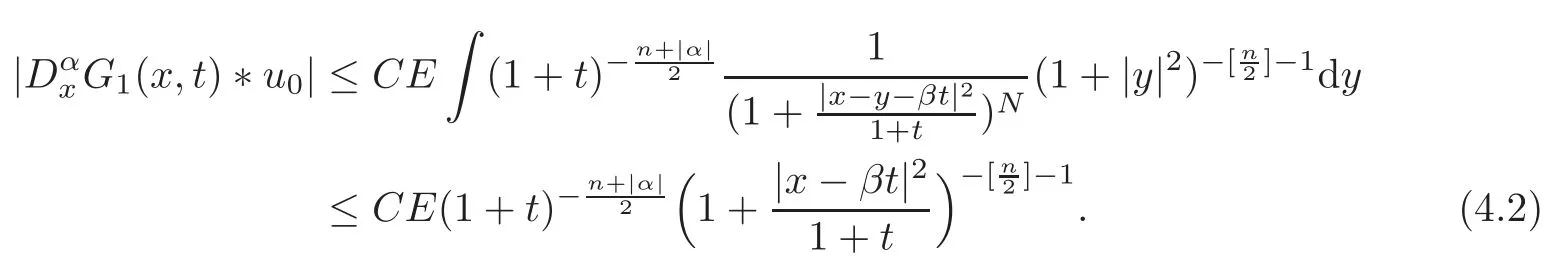
ProofFrom(2.6),we have

From(3.1)and Lemma 3.4,we have

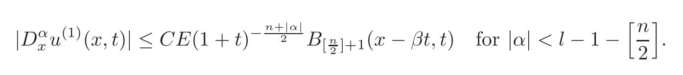
From(3.7),when|γ|＞,we have

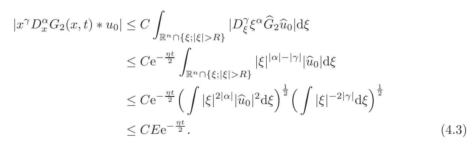
If|α|＜l−1−,we have

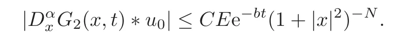
From Lemma 3.2 and(4.4),we have

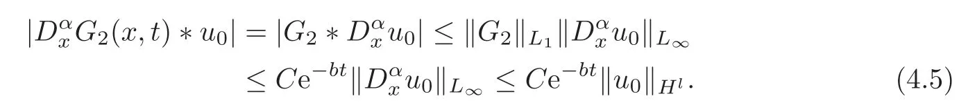
Taking|γ|=2Nin(4.3),from(4.3)and(4.5),we have

From Lemma 3.3,we get

From(4.2)and(4.6),we get our result.

Lemma 4.2For m＞1,if

then

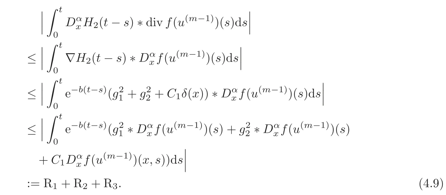
ProofBecause(u)=,we have

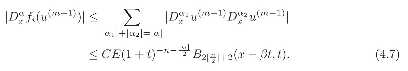
We still denote

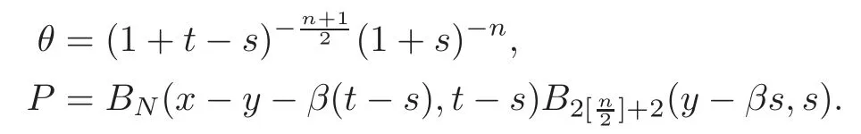
From Lemmas 3.1,3.5 and(4.7),we have

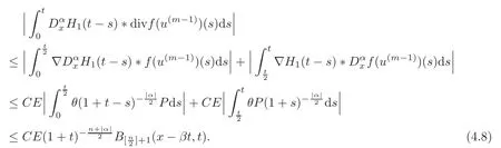
From Lemma 3.2,we have

From Lemma 3.6 and(4.7),we have

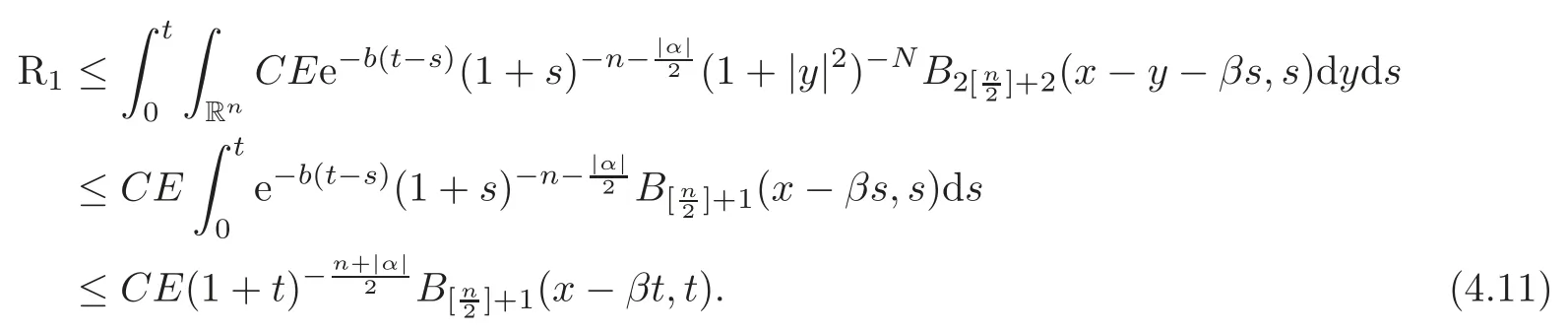
From(3.5),(4.7),Lemmas 3.4 and 3.6,we have

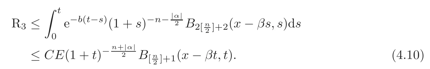
From(3.6),(4.7)and Lemma 3.6,we have

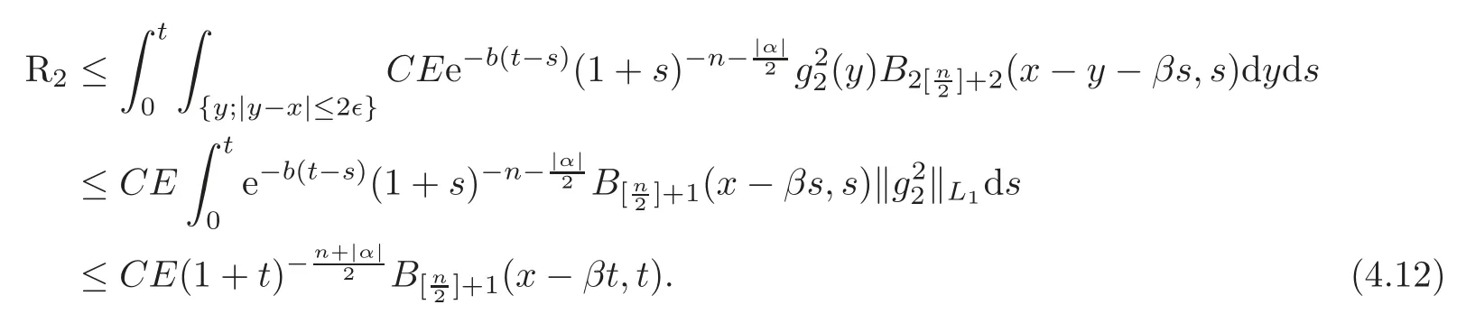
Together with(4.9)–(4.12),we get

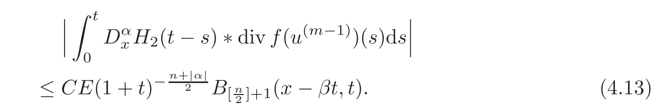
From(2.6),we know that

From(4.8),(4.13)–(4.14)and Lemma 4.1,we get our result.

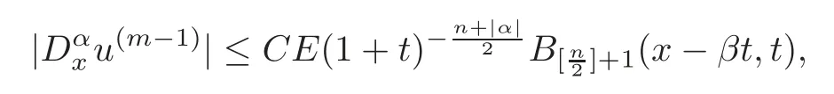
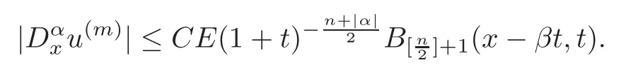
From Lemmas 4.1 and 4.2,using mathematical induction,we know that for allm≥1 and|α|＜l−1−

5 Convergence of the Sequence

In this section,we will prove thatis a Cauchy sequence in a Banach space,and thus it converges to the solution of(1.1)–(1.2).

From[11,Lemma 5.2],it follows that

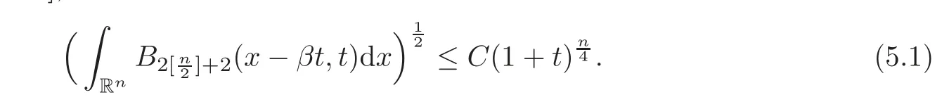
From(4.15)and(5.1),we know(x,t)∈L∞(0,∞;Thusis in a Banach space.We next prove that it is a Cauchy sequence.

Lemma 5.1is a Cauchy sequence in L∞(0,∞;

ProofFrom(2.6),satisfies the following equation

Thus

Set=−(x,t).Then

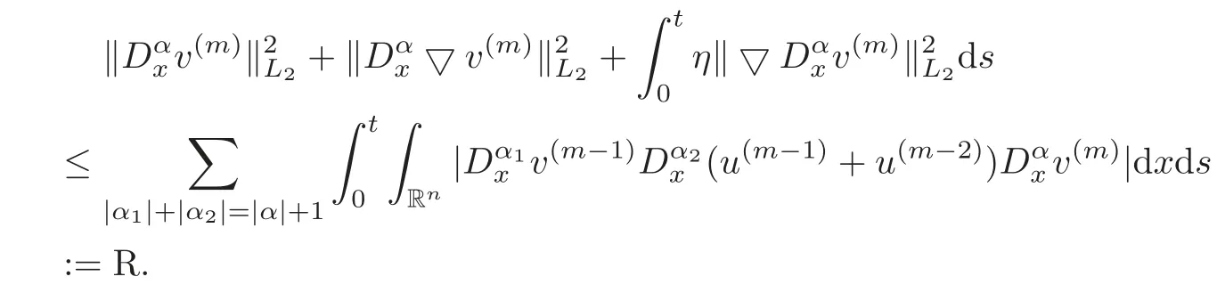
Multiplyingin the two sides of(5.3)and integrating with respect toxin Rn,we get

Whenm≥2,from(2.6)we have(x,0)=0.Thus form≥3,we have

From(4.15),we know

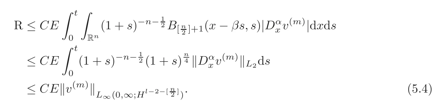
IfCE＜1,from(5.4)we know thatis a Cauchy sequence in Banach spaceL∞(0,∞;and thus it converges to the solution to(1.1)–(1.2).

6 Conclusion

Theorem 6.1If=E,l＞1+≤CE(1+with E small enough,then(1.1)–(1.2)have a global solution in time u(x,t),for|α|≤l−−2,satisfying

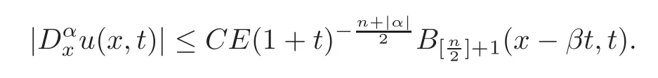
Remark 6.1The solution has the same decay rate as the heat kernel,so our estimation must be optimal.

Remark 6.2The solution decays much faster away along the characteristic linex=βt,so we can say that the solution propagates along the characteristic line.It coincides with the physical phenomenon.

[1]Benjamin,T.B.,Bona,J.L.and Mahony,J.J.,Model equations for long waves in nonlinear dispersive systems,Phil.R.Soc.London,Ser.A,272,1972,47–78.

[2]Avrin,J.and Goldstein,J.A.,Global existence for the Benjamin-Bona-Mahony equations,Nonlinear Anal.,9,1985,861–865.

[3]Goldstein,J.A.and Wichnoski,B.J.,On the Benjamin-Bona-Mahony equation in higher dimensions,Nonlinear Anal.,4,1980,861–865.

[4]Guo,B.L.,Initial boundary value problem for one class of system of multidimensional inhomogeneous GBBM equations,Chinese Ann.Math.,8B(2),1987,226–238.

[5]Albert,J.,On the decay of solutions of the generalized Benjamin-Bona-Mahony equation,J.Mah.Math.Analysis Applic.,141,1989,527–537.

[6]Biler,P.,Long time behavior of solutions of the generalized Benjamin-Bona-Mahony equation in two space dimensions,Diff.,Integral Eqns.,5,1992,891–901.

[7]Fang,S.M.and Guo,B.L.,Long time behavior for solution of initial-boundary value problem for one class of system with multidimensional inhomogeneous GBBM equations,Appl.Math.Mech.,26(6),2005,665–675.

[8]Zhang,L.H.,Decay of solutions of generalized Benjamin-Bona-Mahony-Burgers equations inn-space dimensions,Nonlinear Analysis,25,1995,1345–1369.

[9]Fang,S.M.and Guo,B.L.,The decay rates of solutions of generalized Benjamin-Bona-Mahony equations in multi-dimensions,Nonlinear Anal.,69,2008,2230–2235.

[10]Wang,W.K.and Yang,T.,The pointwise estimate of solutions of Euler equation with damping in multidimensions,J.D.E.,173,2001,410–450.

[11]Liu,T.P.and Wang,W.K.,The pointwise estimates of diffusion wave for the Navier-stokes systems in odd multi-dimensions,Commum.Math.Phys.,196,1998,145–173.