
Simulations of ice jam thickness distribution in the transverse direction*
2014-06-01 12:30:01WANGJun王军SHIFayi施发义CHENPangpang陈胖胖
水动力学研究与进展 B辑 2014年5期
关键词:王军
WANG Jun (王军), SHI Fa-yi (施发义), CHEN Pang-pang (陈胖胖)
School of Civil Engineering, Hefei University of Technology, Hefei 230009, China,
E-mail: junwanghfut@126.com
WU Peng, SUI Jueyi
Environmental Engineering, University of Northern British Columbia, Prince George, British Columbia, Canada
Simulations of ice jam thickness distribution in the transverse direction*
WANG Jun (王军), SHI Fa-yi (施发义), CHEN Pang-pang (陈胖胖)
School of Civil Engineering, Hefei University of Technology, Hefei 230009, China,
E-mail: junwanghfut@126.com
WU Peng, SUI Jueyi
Environmental Engineering, University of Northern British Columbia, Prince George, British Columbia, Canada
(Received November 14, 2013, Revised July 2, 2014)
River ice often forms in the cold regions of northern hemisphere which can lead to ice jams (or ice dams). Water level can be significantly raised due to ice jams. As a consequence, disastrous ice flooding may be resulted, such as the ice jam flooding in the Nechako River in Prince George in winter 2007-2008. In the present study, the equations describing the ice jam thickness in the transverse direction are derived. The impact of the secondary vortex is considered while the cohesive force within ice cubes is neglected in the model. The relationship between the parameter β and the total water depth is established based on the assumption that all other variables except the velocities are kept constant on the same cross section. By using the parameter β and the developed equations, the ice jam thickness in the transverse direction can be predicted. The developed model is used to simulate the ice jam thickness in the transverse direction at the Hequ Reach of the Yellow River in China. The simulated ice jam thicknesses agree well with the field measurements on different cross sections.
ice jam thickness, secondary vortex, cohesive force, transverse distribution
Introduction
The ice jam is an important issue for rivers and it can lead to ice flooding with major social, economic impacts in cold regions. The ice jam alters the hydraulics of an open channel by imposing extra boundaries, and increasing the roughness coefficient as compared to the ice free case[1], resulting in a significant rise of the water level. With the formation of the ice jam, some extreme flood events may occur, with a huge damage to the property and infrastructure. For example, the ice jam is a major cause of flooding in Canada. In Alberta, Canada, the ice jam flooding is an annual concern for the provincial government, while in the province of New Brunswick, Canada, St John River is characterized by repeated ice jam floodings (Environment Canada, 2013). In Asia, the ice jam is also a source of floodings in central and northern regions of China. For example, the break-up of Yellow River is an annual event across China for a long time[2].
Although the ice jam is important for the flood control but it is very difficult to be predicted and measured. Very limited data are available about the ice jam formation and river breakup. Healy and Hicks[3]provided some experimental data for the ice jam formation. With respect to Canadian rivers, Beltaos et al.[4-6]investigated the formation and release of ice jams, and reviewed some models. Beltaos[7]pointed out some potential problems in the study of ice jams. A research group led by Dr. Hicks[8,9]has been continuously working on the monitoring ice jams and acquiring related data in the last few years. She also made an excellent review on the river ice problems around the world[10]. However, the dynamic evolution of the ice jam involves various parameters, related with hydraulic, thermal and boundary conditions. A precise prediction of ice jams is difficult, if not impossible.

1. Model and simulation of thickness distribution
1.1Assumptions and basic equations of the model
Ice jams are formed by ice blocks and frazils accumulated under the ice cover. The size of the ice particles normally varies widely and is much smaller as compared to the width of rivers. So, in the simulation of the thickness of ice jams, the continuous assumption is valid[22]. Beltaos[21]derived the 1-D ice thickenss equations based on the continuous assumption and the static equilibrium of ice jams. However, since the force distribution in the transverse direction is not considered in the derivation, his model for determining the ice jam thickness is limited to the calculation of the jam thickness in a prismatic rectangular channel. Many field observations indicate that the thickness of the ice jam in the transverse direction varies significantly from the riverbank to the main channel. Obviously, the model developed by Beltaos cannot be used to predict the transverse thickness distribution on each cross section.

Fig.1 Stresses on an element of an ice jam cube[21]
In Fig.1, one finite element of ice cube is separated and analyzed, in which, x is the direction of the flow (or the longitudinal direction), y is the vertical direction normal to the water surface and z is in the transverse direction. Following Beltaos’[21]analysis of the 1-D thickness, the following equations for the balance of an ice jam can be derived.


where s'x, s'yand s'zare the normal pressure in x, y and z directions, respectively, which also include the static pressure, τx'y, τ'yz, τx'zare the shear stresses, γ' is the specific gravity of ice, equal to ρig(1-pJ) when the ice body is above the water surface, and equal to ρig(1-pJ)+ρgpJwhen the ice body is under the water surface, ρ is the mass density of water, ρiis the mass density of ice, pJis the porosity of the ice jam, which is a constant with a value of 0.4.
These three equations are integrated in x, y and z directions, respectively, and the following equations are obtained. However, since the channel cross section is normally not rectangular, the secondary vortex in the transverse direction also needs to be considered in the equations.


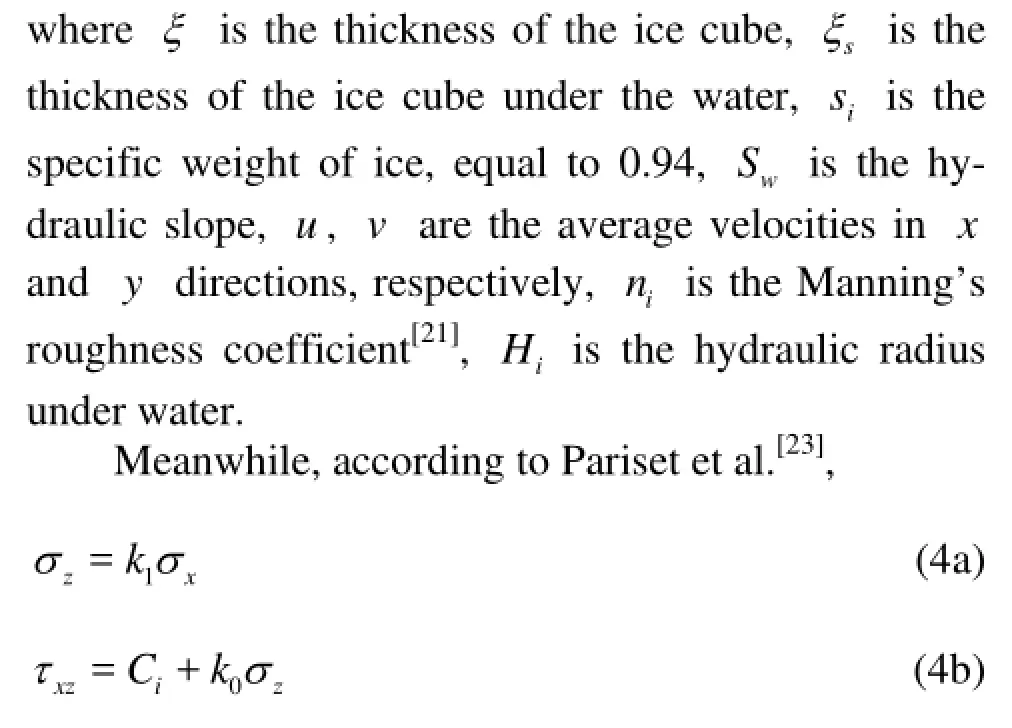
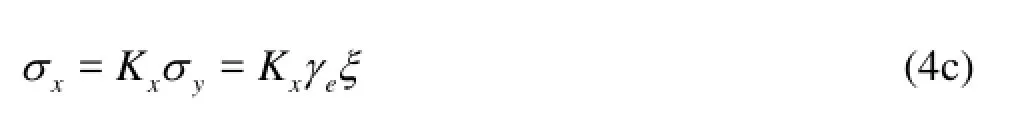
in which, τiand τjcan be calculated as where k0=tanφ, equal to 1.14[21], φ is the inner friction slope of ice cubes, k1is the coefficient of the lateral trust, which is equal to 0.28 here[21], Kxis a coefficient and is assumed to be equal to the passive earth pressure, 6.3[21]and γe=0.5si(1-si)(1-pJ)ρg.
According to Beltaos[21], compared to the inner friction stress, the cohesive stress can be neglected, which means that Ci=0. Based on this assumption and combining Eqs.(2) and (4), the following equation can be obtained.

Equation (5) can then be solved as follows

Equation (8) describes the thickness distribution of the ice jam in the transverse direction. Compared to previous studies, the secondary vortex is considered in this equation which is crucial for the determination of the thickness of the ice jam in the transverse direction.
1.2Analysis of variables
On the same cross section, the hydraulic S is assumed to be constant, so the value of α can also betreated as a constant in the analysis. From Eq.(8), it can seen that under the same thermal condition, the difference in the thickness of the ice jam on the same cross section is mainly determined by the variable β. The ratio of β at different time scales is

Table 1 Hydraulic parameters used in the calculation

Combining Eq.(3) with Eq.(9), we obtain

Based on the analysis of Wu[24], we come to the following relationship.


Fig.2 Hequ Reach of the Yellow River, China
On the same cross section, under the same thermal condition, all variables except the velocity have very little fluctuations, and they can be considered as constant. For wide and shallow rivers, we have Hi≈h/2, V2=4ghSw/f0, f0is the composite friction coefficient, equal to 0.25 according to the field data. Equation (12) is derived by combining Eqs.(10) and (11). The values of some related parameters for the calculation are shown in Table 1.

where hi1, hi2are the total water depth on the same cross section.

Table 2 Calculated β values on different dates on Longkou cross section 1

Table 3 Calculated β values on different dates on Yingzhantan cross section 2
It can be noted from Eq.(12) that the value of β is directly related with the total water depth. In rigid winter times, the flow conditions can be significantly different as compared to the free surface. It is extremely hard to measure the velocity under the ice jam. On the other hand, the water depth measurement is easier compared to the velocity measurement. So by using Eqs.(8) and (12), the ice jam thickness on the transverse direction can be calculated based on the field data.
2. Model validations and result analysis
The Hequ Reach of Yellow River is located in the middle reaches of the Yellow River, as shown in Fig.2. In winter from late November to early March next year, due to the cold air temperatures in the winter, an enormous amount of frazil ice is generated in the open channel upstream of the Hequ Reach. As a direct consequence, the Hequ Reach experienced over 100 d jamming each winter between 1982 and 1991[2,25]. During this period of 9 years, a great number of field measurements of the water level and the frazil jam thickness on several cross sections were made. In this study, the field data from these measurements are used to validate the developed model for the thickness distribution of the ice jam in the transverse direction.
2.1The value of β
By using the field data measured from 1985 to 1992, β can be calculated from Eq.(8). Then based on Eq.(12), the values of β at the approximate time scales under the same thermal conditions can be calculated. The field data from four cross sections are used to validate the proposed equation. Tables 2 through 5 show the calculation results of β on Longkou, Yingzhantan, Beiyuan and Nanyuan cross sections, respectively. However, due to the limitation of the field data, some of β values in Tables 2 through 5 cannot be obtained.
2.2Result analysis
By using the value of β acquired from Tables 2 through 5, several simulations of the thickness distribution of the ice jam in the transverse direction are conducted. The simulation results by using Eq.(8) are compared with the field measurements on different cross sections. Figures 3, 4, 5 and 6 show some simulation results from these simulations.
From these figures, one can see that the calculated ice thickness values in the transverse direction agree in general well with the field measurements. However, at some measuring points on each cross section, the calculated jam thicknesses deviate from the field measurements, such as the simulation results for 26th February 1986 on Yingzhantan cross section (Fig.4) and 16th February 1991 on Nanyuan cross section (Fig.6). The possible reasons for deviations may be as follows: in the development of the equation fordeterminingβ, the thermal conditions are assumed to be the same across the simulated cross section. However in the field, the thermal conditions in the transverse direction on each cross section are not uniform although the variation is not great, since the flow velocity in the main channel is greater than that near the river bank.. Also, the field measurements were carried out from the left bank to the right bank (facing downstream), as noticed by the 5th author, and it took about 4 h to complete measurements for each cross section. During this 4 h period, the thermal conditions for both the ice jam and the flowing water might not be the same.

Table 4 Calculatedβvalue on different dates on Beiyuan cross section 3
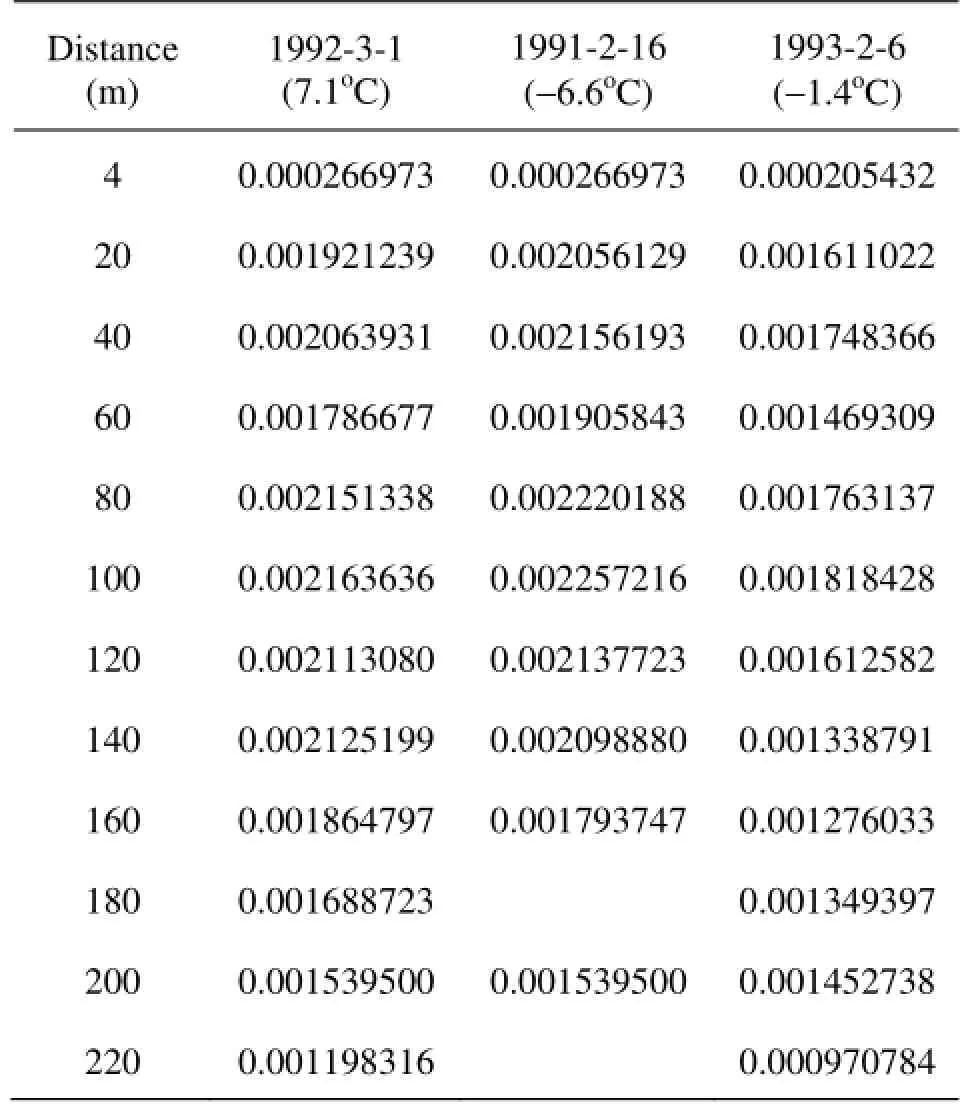
Table 5 Calculated β value on different dates on Nanyuan cross section 4
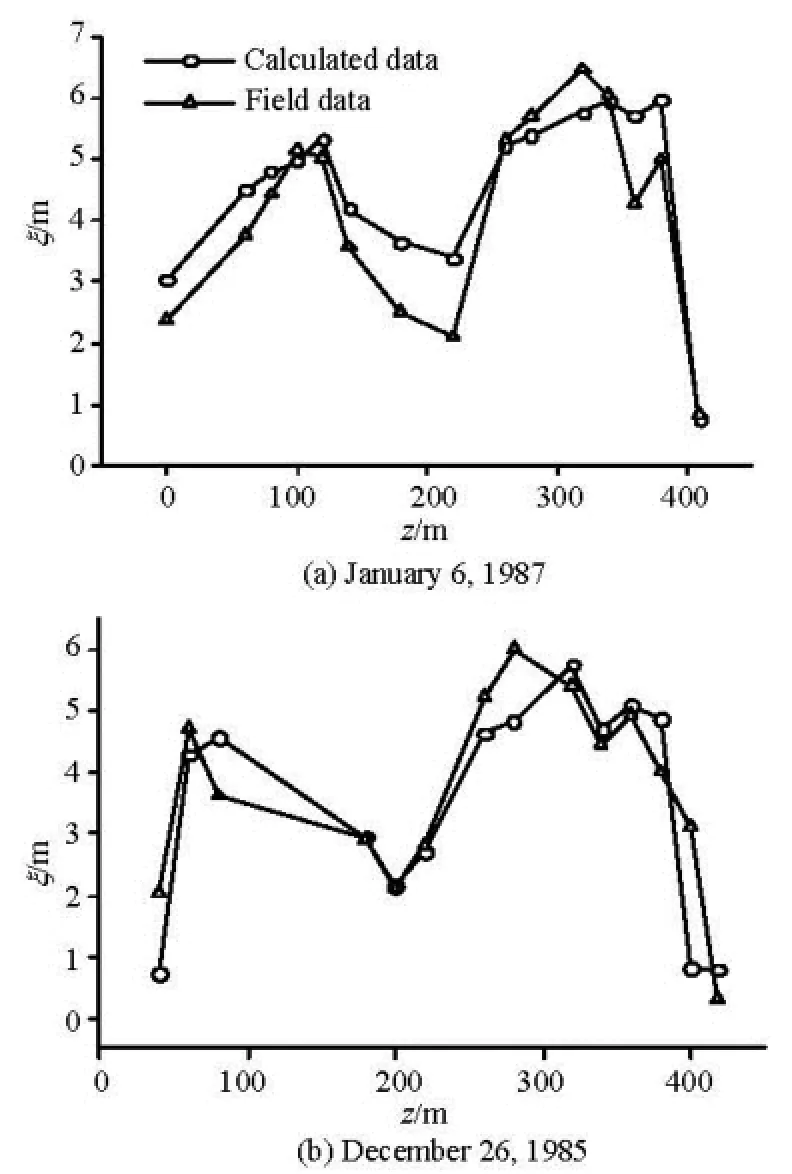
Fig.3 The calculated thicknesses distribution of ice jam compared to field measurements on the Longkou cross section 1 (S=1.52× 10⁻³)w

Fig.4 The calculated thicknesses distribution of ice jam compared to field measurements on the Yingzhantan cross section 2 (Sw=10-3)
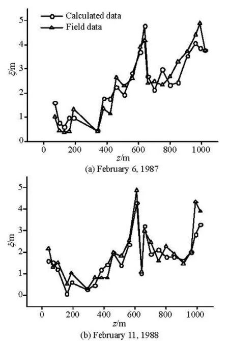
Fig.5 The calculated thicknesses distribution of ice jam compared to field measurements on the Beiyuan cross section 3 (Sw=10-3)

Fig.6 The calculated thicknesses distribution of ice jam compared to field measurements on the Nanyuan cross section 4 (Sw=0.32× 10⁻³)
In overall, the simulated thickness distributions of the ice jam in the transverse direction on each crosssection agree well with the field measurements. The developed model can be used to determine the thickness distribution of ice jams at the Hequ Reach of the Yellow River, and we do hope that this model can be applied to other rivers. This model could be served as a step stone for the development of a 3-D hydrodynamics model for simulating the ice jam process.
3. Conclusion
Based on the static equilibrium of an ice jam, a model is developed to determine the thickness distribution of ice jams in the transverse direction. The secondary vortex is considered in this model. On the same cross section, the difference of the ice jam thickness can be attributed to value β, which can be determined by using the water depth on the cross section. It is reasonable to assume that the thermal conditions are constant on the same cross section. The impact of variable β on the thickness distribution under similar thermal conditions is discussed. From the comparison between the field data and the calculated results, a good agreement is seen on all the four cross sections, except at some points with some deviations. It is concluded that the equation can be used to predict the thickness distribution of ice jams in the transverse direction.
Acknowledgement
The authors gratefully acknowledgement the help from the Foundation and staff from Hefei University of Technology.
[1] SHEN H. T., WANG D. Under cover transport and accumulation of frazil granules[J]. Journal of Hydraulic Engineering, ASCE, 1995, 121(2): 184-195.
[2] SUI J., KARNEY B. and SUN Z. et al. Field investigation of frazil jam evolution–A case study[J]. Journal of Hydraulic Engineering, ASCE, 2002, 128(8): 781-787.
[3] HEALY D., HICKS F. Experimental study of ice jam formation dynamics[J]. Journal of Cold Regions Engineering, 2006, 20(4): 117-139.
[4] BELTAOS S. Discussion of “smoothed particle hydrodynamics hybrid model of ice-jam formation and release”[J]. Canadian Journal of Civil Engineering, 2010, 37(4): 657-658.
[5] BELTAOS S., TANG P. and ROWSELL R. Ice jam modelling and field data collection for flood forecasting in the Saint John River[J]. Hydrological Processes, 2012, 26(17): 2535-2545.
[6] BELTAOS S., CARTER T. and ROWSELL R. Measurements and analysis of ice breakup and jamming characteristics in the Mackenzie Delta, Canada[J]. Cold Regions Science and Technology, 2012, 82: 110-123.
[7] BELTAOS S. Progress in the study and management of river ice jams[J]. Cold Regions Science and Technology, 2008, 51(1): 2-19.
[8] GHOBRIAL T., LOEWEN M. and HICKS F. Laboratory calibration of upward looking sonars for measuring suspended frazil ice concentration[J]. Journal of Cold Regions Science and Technology, 2012, 70: 19-31.
[9] DOW K., STEFFLER P. and HICKS F. Analysis of the stability of floating ice blocks[J]. Journal of Hydraulic Engineering, ASCE, 2011, 137(4): 412-422.
[10] HICKS F. An overview of river ice problems[J]. Journal of Cold Regions Science and Technology, Special Issue on River Ice, 2009, 55(2):175-185.
[11] LI Zhi-jun, HAN Ming and QIN Jian-min et al. States and advances in monitor of ice thickness change[J]. Advances in Water Science, 2005, 16(5): 753-757(in Chinese).
[12] SUN Zhao-chu, WANG De-sheng and WANG Zhaoxing. The discussion of ice thickness calculation models[J]. Journal of Hydraulic Engineering, 1985, (1): 54-60(in Chinese).
[13] SUI J., WANG J. and BALACHANDAR R. et al. Accumulation of frazil ice along a river bend[J]. Canadian Journal of Civil Engineering, 2008, 35(2): 158-169.
[14] WANG J., SUI J. and CHEN P. et al. Mechanisms of ice accumulation in a river bend–An experimental study[J]. International Journal of Sediment Research, 2012, 27(4): 521-537.
[15] HEALY D., HICKS F. Experimental study of ice jam thickening under dynamic flow conditions[J]. Journal of Cold Regions Engineering, 2007, 21(3): 72–91.
[16] NOLIN S., ROUBTSOVA V. and MORSE B. Smoothed particle hydrodynamics hybrid model of ice-jam formation and release[J]. Canadian Journal of Civil Engineering, 2009, 36(7): 1133-1143.
[17] SHEN H. T. Mathematical modeling of river ice processes[J]. Cold Regions Science and Technology, 2010, 62(2): 3-13.
[18] WANG Jun, CHEN Pang-pang and JIANG Tao et al. The simulation of ice accumulation under ice cover[J]. Journal of Hydraulic Engineering, 2009, 40(3): 348-354(in Chinese).
[19] WANG Jun, CHEN Pang-pang and SUI Jueyi. Numerical simulation of ice jams in natural channels[J]. Journal of Hydraulic Engineering, 2011, 42(9): 1117-1121(in Chinese).
[20] CARSON R., BELTAOS S. and GROENEVELD J. Comparative testing of numerical models of river ice jams[J]. Canadian Journal of Civil Engineering, 2011, 38(6): 669-678.
[21] BELTAOS S. River ice jams[M]. Highlands Ranch, Colorado, USA: Water Resources Publications, 1995, 105-146.
[22] SHEN Hong-dao. River ice study[M]. Zhengzhou, China: Yellow River Water Conservancy Press, 2010, 67-103(in Chinese).
[23] PARISET E., HAUSSER R. and GAGNON A. Formation of ice covers and ice jams in rivers[J]. Journal of the Hydraulics Division, ASCE, 1966, 92(6): 1-24.
[24] WU Chang-jun. The study of flow field and ice accumulation of ice jams under ice cover in a curved channel[D]. Doctoral Thesis, Hefei, China: Hefei University of Technology, 1993(in Chinese).
[25] SUI J., KARNEY B. and Fang D. Variation in water level under ice-jammed condition–Field investigation and experimental study[J]. Nordic Hydrology, 2005, 36(1): 65-84.
10.1016/S1001-6058(14)60085-8
* Project suppotted by the National Natural Science Foundation of China (Grant Nos. 51379054, 50979021).
Biography: WANG Jun (1962-), Male, Ph. D., Professor
SUI Jueyi, E-mail: jueyi.sui@unbc.ca
猜你喜欢
Acta Mathematica Scientia(English Series)(2022年2期)2023-01-09 10:57:00
红蜻蜓·低年级(2021年9期)2021-09-22 13:23:30
好孩子画报(2020年5期)2020-06-27 14:08:05
音乐天地(音乐创作版)(2019年10期)2020-01-06 11:51:54
活力(2019年19期)2020-01-06 07:34:36
作文周刊·小学一年级版(2019年32期)2019-10-15 13:54:37
作文周刊·小学二年级版(2019年32期)2019-10-15 13:33:16
中华建设(2019年4期)2019-07-10 11:50:58
水动力学研究与进展 B辑(2018年2期)2018-05-14 01:43:20
水动力学研究与进展 B辑(2015年6期)2015-12-01 02:12:14

- 水动力学研究与进展 B辑的其它文章
- Experimental and numerical study on hydrodynamics of riparian vegetation*
- Vadose-zone moisture dynamics under radiation boundary conditions during a drying process*
- A numerical analysis of the influence of the cavitator’s deflection angle on flow features for a free moving supercavitated vehicle*
- Retard function and ship motions with forward speed in time-domain*
- Stability of fluid flow in a Brinkman porous medium-A numerical study*
- Sediment rarefaction resuspension and contaminant release under tidal currents*