Evaluation of Three Harvest Control Rules for Bigeye Tuna(Thunnus obesus)Fisheries in the Indian Ocean
TONG Yuhe,CHEN Xinjun,,and Dale Kolody
1)Fisheries Research Institute of Hainan Province,Haikou 570206, P.R.China
2)College of Marine Sciences,Shanghai Ocean University,Shanghai 201306,P.R.China
3)The Key Laboratory of Sustainable Exploitation of Oceanic Fisheries of Ministry of Education,Shanghai Ocean University,Shanghai 201306,P.R.China
4)Indian Ocean Tuna Commission Secretariat,PO Box 1011, Floor 2, Le Chantier Mall,Victoria,Seychelles
© Ocean University of China,Science Press and Spring-Verlag Berlin Heidelberg 2014
1 Introduction
Bigeye tuna,Thunnus obesus,is one of the top predators in the ecosystems of the Indian Ocean.It is a sashimi-quality tuna of considerable economic importance,and its importance is likely to increase with the decline of the bluefin tuna fisheries(Safina and Klinger,2008; MacKenzieet al.,2009).Bigeye tuna is harvested by fleets from several countries using various fishing gear,including longline and purse seine which accounts for more than 97% of the total landing.This data is provided by the Indian Ocean Tuna Commission(IOTC).Longline fisheries target bigger fish in deeper water(usually >100 m)and yield the highest catch in mass,while purse seine fisheries targeting skipjack and yellowfin tuna,often land small bigeye tuna as a by-catch when using fish aggregating devices(FADs)(IOTC Secretariat,2005).
The IOTC is responsible for the management of bigeye tuna.While operational reference points have yet to be agreed by the commission,there is a general expectation that the spawning stock biomass(SSB)should not fall much below a level that can support the maximum sustainable yield(MSY)(i.e.,SSBmsy)as prescribed in the UN Fish Stocks Agreement(IOTC,2010).However,there is no harvest strategy which prescribes what action should be taken if theSSBfalls belowSSBmsy.The latest IOTC assessment suggests that the bigeye tuna stock is not likely to be overfished(SSB2009>SSBmsy)at present,but the stock is near to full exploitation,and an uncertainty in the stock assessment suggests that these reference points could be exceeded(Kolodyet al.,2010).Meanwhile,the updated IOTC resolution states that bigeye tuna stocks might have been over or fully exploited in recent years(IOTC,2010).The total annual catch decreased from its peak of around 150000 t in 1999 to 100000 t in 2009,and in particular the Japanese standardized catch per unit effort(CPUE)for longline fishery declined by more than half from 1977 to 2009(Okamoto and Shono,2010).Although the most recent total catch is likely to be below MSY(114000 t,Kolodyet al.,2010),there is considerable uncertainty in stock assessment and landing data.Therefore,managers should plan for appropriate action before or when the fishery has become over-exploited.The updated IOTC resolution has noted the importance of applying a precautionary approach to managing bigeye tuna(IOTC,2010).It has called for an understanding of how the stock of bigeye tuna may respond to different management strategies in the face of uncertainty on current stock status and key life history characteristics.
A fully specified management procedure includes a harvest control rule(HCR),data collection and analysis methods.The HCR is designed to be robust to uncertainty and to have a high probability of achieving a reasonable balance between competing biological and socioeconomic objectives(Holland,2010).Monte Carlo simulations are usually used in an operating model to simulate population dynamics with a broad range of uncertainty,including observation,process,implementation and model specification errors(Butterworth,2007).HCRs have been developed for many fisheries including tuna(Fromentin and Kell,2008; Zhanget al.,2013),but few have been evaluated for international fisheries(Zhanget al.,2013).
In this study,we assessed the short,medium and long term performances of three constant HCRs with Monte Carlo simulations under pre-specified management objectives for bigeye tuna.To be consistent with Stock Synthesis III(SS3)based on stock assessment(Kolodyet al.,2010),we identified three groups of stock assessment outputs representing different scenarios and assumptions to cover possible uncertainty in the stock assessment.The three groups included low,medium and high productivity.They represented the stock assessment outputs considered to have the most uncertainty,and thus might cover the‘true’ population dynamics.Although the framework developed in this study is for the bigeye tuna fishery in the Indian Ocean,it also has implications for other fisheries.
2 Methods
The methods can be divided into three sections:i)an operating model which simulates fish population and fishery dynamics,and alternative hypotheses that encompass the major uncertainty; ii)HCRs,the decision algorithms which produce a total allowable catch(TAC)recommendation as a function of the simulated data; and iii)performance measures which include statistics for stock and fishery indicators,and probabilities of achieving/violating management objectives for the simulated performance of the HCRs.
2.1 The Operating Model and Its Uncertainty
An age-structured population dynamics model with an annual time-step was used to make stochastic forward projections.The current stock status and biological parameters were derived from three specifications of the most recent bigeye tuna stock assessment(Kolodyet al.,2010).Population was represented by 16 year classes(i.e.,0–15+years).Four fishing fleets,combined longline(LL),purse seine free school sets(PSFS),purse seine log sets(PSLS)and all others(Other),were selected for their different fishing methods to reflect capacity and fishing targets,including size of fish.Catches were extracted using the Baranov catch equation.The Beverton-Holt stockrecruitment relationship with steepness fixed at 3 values(h,Tables 1 and 2)and a constant standard deviation for recruitment(σR,Table 2)were assumed.Spawning stock biomass(SSB)was assumed to be proportional to the mass of matured fish.Biological parameters,including length-at-age,weight-at-age,maturity-at-age and naturalmortality(M)-at-age relationships were assumed to be stationary within each simulation(Fig.1),however M varied among the 3 operating models.
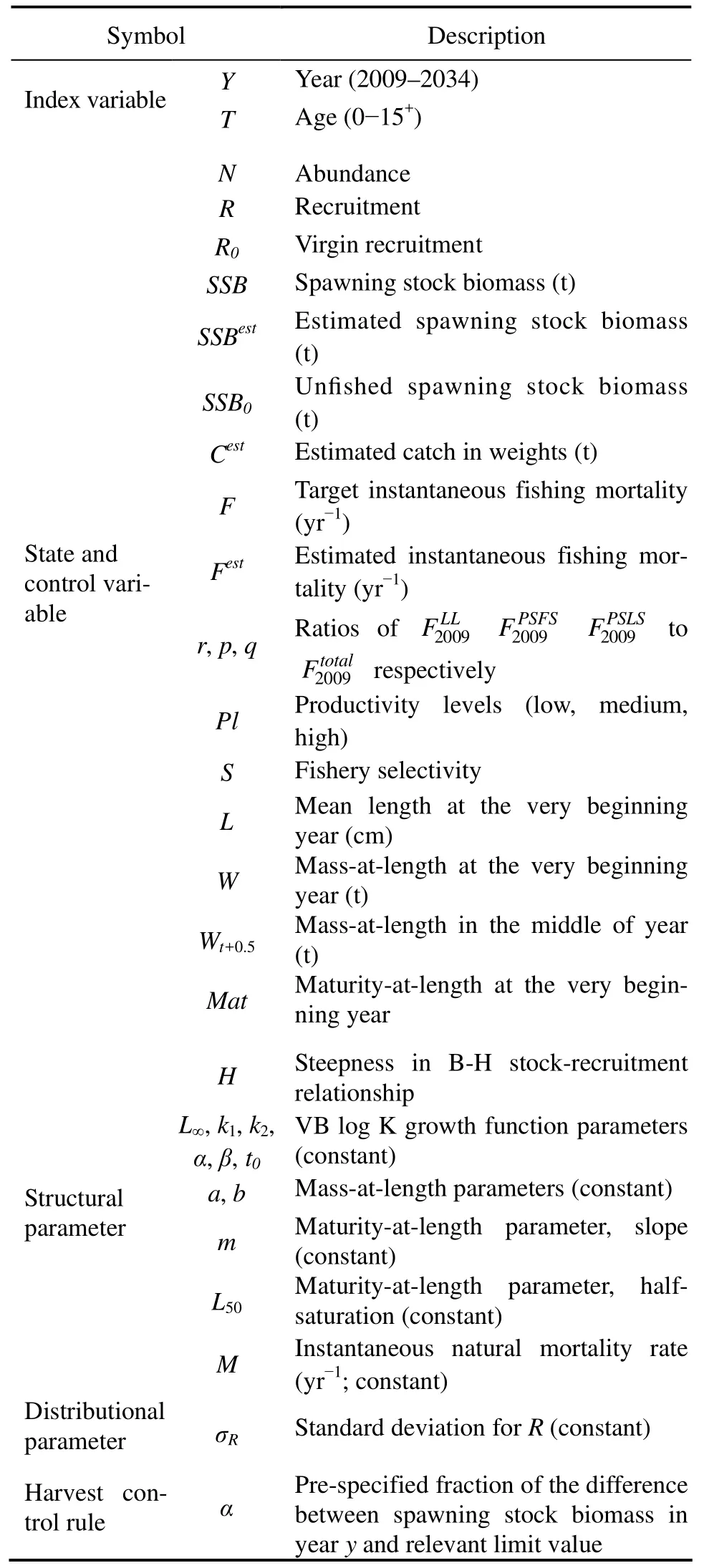
Table 1 Symbols and descriptions of variables used in the stochastic simulation model

Table 2 Values defined for various parameters used in thestochastic simulation model
The notation,operating model equations and model parameters are detailed in Tables 1,2 and 3,respectively(IOTC,2008),which come from the IOTC database at website(www.iotc.org/English/data/databases.php).The operating model included three Maximum Posterior Density(MPD)specifications(Kolodyet al.,2010),which were selected to span the range of productivity that was considered to be plausible in the assessment subsequently referred to as low,medium and high productivity.As such,the framework was intended to compare the general performance and robustness of a range of policy options,and to select the appropriate HCR.

Fig.1 Selectivity-at-age for longline(●),FAD associated purse seine(■),unassociated purse seine(▲)and other fisheries(×)at low,medium and high productivity from Stock Synthesis III(SS3).
As described below,the feedback-based HCRs require estimates ofSSByand instantaneous fishing mortality(Fy)to produce TAC recommendations.We used specific estimation errors(biasFand biasSSB,Tables 1–3)for each operating model,which ensures that the population estimates are initially consistent with the historical data for each of the three productivity scenarios.As the actual productivity level is unknown,three possible levels are set in our study and the results for each harvest policy are summarized.The bias term was intended to prevent the simulation from having unrealistically informative data.The bias term could also reflect bias in stock assessment at different productivity levels caused by inappropriate parameter estimation,e.g.,natural mortality rate.There was no implementation error(i.e.,the catch removed was always equal to the TAC)and no observed error(i.e.,the estimated catch was equal to the catch removed)in catch data.Apart from the optimal strategy identified,the sensitivity to implementation error was evaluated.Uncertainty in the parameters of the stock-recruitment relationship was also considered.As the aim of this study is to evaluate the performance of the HCRs,the unincorporated uncertainty is not likely to influence the qualitative results which have been proven in the previous studies of Irwinet al.(2008)and Pomaredeet al.(2010).For each of three productivity scenarios,250 Monte Carlo simulation runs were conducted,with each simulation run covering 25 years.The MPD stock status for 2009 was used as the starting point in the simulation(Table 4; Fig.2).

Table 3 Equations used in the stochastic simulation model

Table 4 Management scenarios and associated parameter values
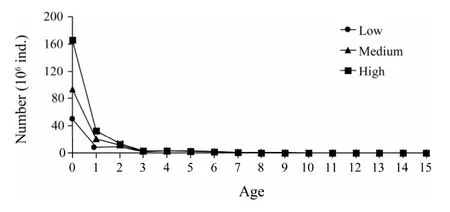
Fig.2 Number-at-age at low,medium and high productivity from Stock Synthesis III(SS3).
2.2 Setting Harvest Control Rules
Three HCRs,Constant Fishing Mortality Rate(CF),Constant Catch(CC)and Constant Escapement(CE),were evaluated in this study(Fig.3).The CF strategy is required to specify a fishing mortality rate which remains constant over time for each fleet and which,if widely implemented,can often achieve proper stock biomass and long-term yield with low management cost(Walters and Parma,1996).In this study,we evaluated five harvest levels from 0.2(defined ase.g.CF_0.2; Table 4)to 0.6 yr−1to represent the protection of stock at different levels.

Fig.3 Graphic representations of constant harvest control rules considered in this study.
There is a significant difference between our constant fishing mortality rule and the commonly used one,in that a ‘true’ fishing mortality rate is estimated from biomass by stock assessment and catch simulated with mean catch at preset levels by Monte Carlo simulations,whereas the commonly used constant fishing mortality rule will be seriously affected if the actual stock assessment errors are large(Willis and Millar,2005).For comparison purposes,keeping a constant fishing effort is also considered,and fisheries management under this rule will not be influenced by stock assessment errors.This CF rule could be applied by controlling the fishing effort,although it has the disadvantage of not solving the fishing effort standardization problem(Maunder and Punt,2004).
A constant catch strategy could provide the industry with greater predictability by avoiding an interannual variation in harvest.However,it may produce low longterm yields and increase the risk of stock being overfished(Hjerne and Hansson,2001).Five catch levels from 60000 to 140000 t are considered,which cover the current catch level and the MSY.In this study,the TAC was abandoned only when stock biomass could not support the annual catch.
A constant escapement strategy,also referred to as a‘fraction/minimum biomass strategy’(Ishimuraet al.,2005),is a conservative way of continuously keeping stock biomass above its minimum exploitable level(Hjerne and Hansson,2001; Deroba and Bence,2008).It can be defined as

whereαis a pre-specified fraction of the difference between spawning stock biomass in yearyand the relevant limit value(SSBL).Five scenarios of this strategy were tested in this study.
2.3 Performance Measures
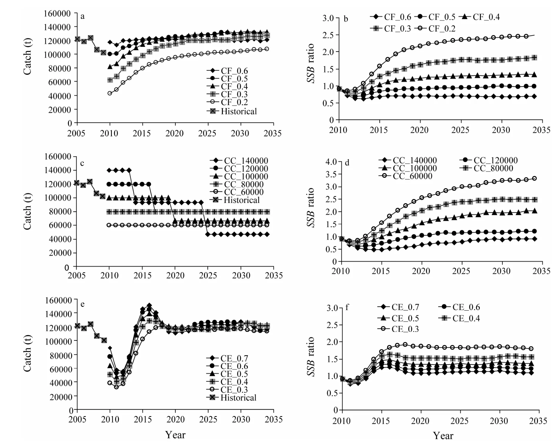
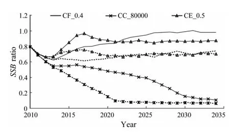
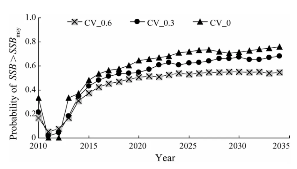
Based on an updated resolution of keeping a stable catch at no more than the MSY level while avoiding overfishing(F>Fmsy)and stock being overfished(SSB 1)Median value(over 250 simulation runs)of the median catch over a 25 year simulation period; 2)Median value(over simulation)of the 25-year interannual catch variability(ICV)was defined as:whereCyis the catch in yeary.A lower value corresponds to a more stable fishery,and is generally preferable for the industry; 3)Median value(over simulation)of the ratio of spawning biomass at the end of the projection years(SSB2034)toSSBmsy; 4)Median value(over simulation)of the ratio of the average spawning biomass over 25 years toSSBmsy; 5)The proportion of years with an annual spawning biomass aboveSSBmsyduring the first 3,10 and 25 years was summarized for all simulations; 6)The proportion of years with an annual catch between 0.8 and 1.0 MSY during the first 3,10 and 25 years was also summarized for all simulations. As the total variance of catch during all projection years is not very meaningful(Puntet al.,2005),ICVis used in our study instead of the coefficient of variance or the standard deviation of an annual catch,to explore the variability of interannual catches.Because most of the scenarios in this study tended to approach equilibrium at the end of 25-year simulations,SSB2034was considered to represent the equilibriumSSB.When calculating the probabilities of achieving management goals,durations of 3 years,10 years and 25 years were used to represent the short,medium and long terms,respectively. According to the management objective and performance measures above,we selected the best strategy for the management measures under consideration using the following criteria:a)the best strategy should ensure the averageSSBaboveSSBmsyor produce the highestSSB,and/or b)the best strategy should achieve the highest average catch if the differences of the average catch were no less than 0.05MSY(around 5600 t in this study; MSY =111195 t; IOTC,2008).Ideally,we prefer to identify a strategy that can satisfy both criteria.However,if none of the strategies can meet both criteria,we would aim to select the strategy that satisfies one of the criteria and does best on the other performance measures as the best strategy. All the scenarios yielded pessimistic results in the first 3 years because of a series of weak year classes in the initial year of 2009.For all CF scenarios,ICVs were low(smaller than 8)(Table 5),and the catches were differentin the first year of 2010,but tended to be constant from 2020(Fig.4a).When comparing the lower constant catch with a range between 95000 t and 105000 t at scenario CF_0.2,the equilibrium catch of other scenarios was between 115000 t and 130000 t after 2020(Fig.4a).TheSSBs behaved similarly from 2015 and increased gradually ifFwas higher than 0.3(Fig.4b). Table 5 Equal weighted values of performance measures derived from 250 simulation runs of three models,for a simulated bigeye tuna fishery with different management strategy scenarios for 25 years of simulation duration Fig.4 Temporal trajectories of median catch and median value of SSB ratio to SSBmsy under different management strategies. TheSSBat the end of the projection year(SSB2034)was critical as all the CF scenarios could eventually result in almost constant catches at differentSSBs.For scenarios CF_0.6 and CF_0.5,SSB2034was only 0.69SSBmsyand 0.98SSBmsy,respectively(Table 5).In contrast,SSB2034reached 1.83SSBmsyand 2.49SSBmsyfor scenarios CF_0.3 and CF_0.2,respectively,which accordingly means thatSSBs were as high as 1.68SSBmsyand 2.24SSBmsy.However,the median catches were lower than that for those two scenarios(CF_0.6 and CF_0.5; Table 5).Scenario CF_0.4 seemed to be optimal,because its median forSSBandSSB2034was more than theSSBmsylevel,and its median catch(around 126000 t)was higher than that obtained for scenarios CF_0.3 and CF_0.2,and was also higher than the 2009 level(101982 t; Table 5; Figs.4a and 4b). The result showed that a higher total allowable catch would result in higher ICVs(Table 5).When the annual catch was at 80000 t,the stock increased from 0.77SSBmsyin the third year(2012)to 2.48SSBmsyin 2034(Fig.4c),and the medianSSBreached 2.20SSBmsy(Table 5).Compared to the other constant catch scenarios(except CC_140000),CC_ 80000 t could achieve a higher median catch(Fig.4c; Table 5).In contrast,CC_140000 t would cause the medianSSBto fall below theSSBmsyduring most of the simulation years(Fig.4d; Table 5).Although CC_60000 could ensure higher stock abundance,the median catch was much lower than CC_80000(Table 5).Thus,of the five constant catch scenarios,scenario CC_80000 was the most desirable. In the constant escapement strategies,the five exploitation rates considered were 0.3 to 0.7 by a step of 0.1 with the limit forSSBpreset at 0.5SSBmsy(Table 4).For all constant escapement scenarios ICVs were very high at more than 16(Table 5).The catch declined from 55000 t in the first year to 37000 t in 2012,then increased to maximum values between 113000 t and 151000 t in 2016,and declined again before 2019(Fig.4e).All constant escapement scenarios produced a steady median catch andSSBafter 2019(Fig.4f).The results also showed thatICVs were higher for the scenarios with higher exploitation rates(Table 5). As medianSSBs were kept above theSSBmsyfor all scenarios,scenarios CE_0.3 and CE_0.4 were not appropriate due to their resultant low catches.For scenario CE_0.5,the median catch was slightly less(around 2000 t)than that of scenario CE_0.6 and slightly higher than that of scenario CE_0.7.However,its medianSSBwas higher than those for scenarios CE_0.6 and CE_0.7,and its ICV was much less than those for scenarios CE_0.6 and CE_0.7(Table 5).This suggests that the scenario of CE_0.5 was the most rational among the five constant escapement scenarios. Among the five scenarios in each of the three groups of constant HCRs considered,optimal choices for the bigeye fishery in the Indian Ocean were scenarios CF_0.4,CC_80000 and CE_0.5,which could result in the medianSSBs being above theSSBmsyand median catches above 80000 t(Table 5).Among these the highest median catch was achieved at 126000 t when fishing mortality was kept at 0.4 yr−1,while the highest medianSSBwas reached at 2.20SSBmsyfor scenario CC_80000.When comparing the above three scenarios using the Kobe II strategy matrix(Table 6),it is not an appropriate choice to keep the escapement rate at 0.5 for the lowest median catch with only a slightly higher probability of achieving theSSBtarget in the medium and long run.Therefore we concluded that the CE_0.5 strategy is not optimal even though it produced higher medianSSBthan CF_0.4(Tables 5 and 6).If the management goal is to harvest more fish,scenarios CF_0.4 should be the choice.However,if the management goal is to focus on conservation,scenario CE_0.5 is the most appropriate because it gives the highest probability of ensuring anSSBgreater than theSSBmsyin the simulation years,especially in the short term(Tables 5 and 6).As environmental change is considered to be one of the major reasons for stock decline(Hilborn and Litzinger,2009; Brander,2010),any optimal harvest rule should also prevent stock from being overfished in areas of low stock productivity because of adverse environmental factors.Scenarios CF_0.4 and CE_0.5 could avoid stock decline with a probability of 90% in the long term at low productivity,while CC_80000 would lead to a rapid decline in fish stocks(Fig.5).We concluded that CF_0.4 was the optimal strategy,as it produced the highest yield,and had a highprobability of reaching theSSBtarget,and avoiding stock collapse when productivity was low.The result shows that scenario CF_0.4 is robust to implementation error.Compared to applying a constant fishing mortality rule at 0.4 yr−1without implementation error,the risk of stock being overfished with a medium implementation error(CV_med =0.3)will be 0.1 higher.Even with a high implementation error(CV_high =0.6),the increased risk of stock being overfished will be lower than 0.2(Table 2; Fig.6). Table 6 Kobe II strategy matrix derived from the management objective grid with equal weighted models described in Table 3 Fig.5 Results for the low producitivity operating model for the ‘true’ median SSB ratio(solid lines)and the 10th percentile SSB ratio(dashed lines)of three optimal management scenarios. Fig.6 Sensitivity analysis to implementation error for scenario CF_0.4 under CV at 0.6(×),0.3(●)and 0(▲). The error of stock assessment may influence interannual variation in harvest,although it is not believed to substantially influence simulation results(Irwinet al.,2008).Managing the bigeye tuna fishery by controlling fishing mortality is not unpopular.For example,the scientific bodies(firstly the Standing Committee on Tuna and Billfish and latterly the Scientific Committee)of one of the world’s largest bigeye tuna fisheries in western and central Pacific Ocean(WCPC),constrained the fishing effort from 2000 after increasing concern about the state of the bigeye tuna fishery(Langleyet al.,2009),although some problems existed after a constant fishing mortality rule was implemented,such as the CPUE standardization and overcapacity.However,according to our sensitivity analysis,such implementation errors could only have a minor impact under a constant fishing mortality rule(Fig.6). It is critical to set TACs for the bigeye tuna fishery in the Indian Ocean for both resource conservation and utilization.Based on the results from our study,the annual catch should be kept at a level lower than that of 2009(100000 t)in the short term.Although the updated resolution stated an ad hoc management strategy of keeping the catch under MSY level(114000 t; IOTC,2010),we believe that the fixed annual catch of around 80000 t is a better choice to allow the management system full control(the indicator signals move below the reference values; Kelly and Codling,2006),while setting MSY as a target catch often results in stock being overfished(Punt,2001).This is because scenario CC_80000 was shown to be optimal when compared with other constant catch scenarios with the weighted result of three productivity models(Table 6).CC_80000 could also have low interannual variability in catch even when productivity is low.In contrast the fishery would have had to close after the 11th simulation year or earlier at an annual catch at 100000 t or more when productivity is low,and the stock would not have recovered until the end of the simulation(Fig.7).This indicates that it is almost impossible for bigeye stock to recover if it collapses to a level of 0.15SSBmsyor lower when productivity is low.This result is consistent with Kolody’s projection which showed that an annual catch at 80% of C2008(around 85000 t)would achieve a 15% lower probability of stock over- exploitation and an 18% lower probability of overfishing than that at C2008(around 106600 t)both in the short term and the medium term(Kolodyet al.,2010). Fig.7 The ‘true’ median SSB ratio to SSBmsy for the high(dashed lines),median(broken lines)and low productivity(solid lines)operating models for scenarios CC_80000(×),CC_100000(●)and CC_120000(▲). Compared to a low TAC in the short term,our result showed that the annual catch could be up to 120000 t in the long term(Figs.4a,4e),because most of the CF and CE scenarios could give a stable long-term yield of around 120000 t after 10 simulation years,which indicates that the stock may be not be being overfished now and that a TAC of 120000 t could be stably yielded after stock recovery.An annual catch of above 120000 t in the short term might not only cause stock collapse under high productivity(Fig.7).Our results also indicated a high risk of stock collapse if the annual catch was around the MSY level,especially when stock productivity was uncertain. However,all the strategies considered in this study for achieving a ‘tolerable’ balance between resource conservation and utilization are subject to further objective interpretation and judgment,and final decisions shall be made by the IOTC in light of further discussion and consideration of its management objectives. Acknowledgements This work is supported by Shanghai Ocean University Graduate School(PhD Dissertation Grant),the National High-tech R&D Program of China(863 Program 2012AA 092303),Project of Shanghai Science and Technology Innovation(12231203900),Industrialization Program of National Development and Reform Commission(2159999),National Key Technologies Research,Development Program of China(2013BAD13B00),and Shanghai Universities First-Class Disciplines Project(Fisheries A). Brander,K.,2010.Impacts of climate change on fisheries.Journal of Marine Systems,79:389-402. Butterworth,D.S.,2007.Why a management procedure approach? Some positives and negatives.ICES Journal of Marine Science,64:613-617. Deroba,J.J.,and Bence,J.R.,2008.A review of harvest policies:Understanding relative performance of control rules.Fisheries Research,94:210-223. Fromentin,J.M.,and Kell,L.T.,2008.Evaluation of the performance and robustness of VPA-based stock assessment and MSY-based management strategy to process error:The Atlantic bluefin tuna case study.Collective Volume of Scientific Papers ICCAT,SCRS/2008/094,64(2):491-506. Hilborn,R.,and Litzinger,E.,2009.Causes of decline and potential for recovery of Atlantic cod populations.The Open Fish Science Journal,2:32-38. Hjerne,O.,and Hansson,S.,2001.Constant catch or constant harvest rate?–The Baltic Sea cod(Gadus morhuaL.)fishery as a modelling example.Fisheries Research,53:57-70. Holland D.S.,2010.Management strategy evaluation and management procedures:Tools for rebuilding and sustaining fisheries.OECD Food,Agriculture and Fisheries Working Papers,No.25.OECD Publishing,67pp,DOI:10.1787/ 5kmd77jhvkjf-en. IOTC Secretariat,2005.A review of the situation of bigeye tuna(Thunnus obesus)in the Indian Ocean.Collective Volume of Scientific Papers ICCAT,57(2):201-217. IOTC,2008.Growth of tropical tunas using the Laslett,Polacheck and Eveson(LEP)method.IOTC-2008-WPTT-09,41pp. IOTC,2010.For the conservation and management of tropical tunas stocks in the IOTC area of competence(Resolution 10/01).Collection of Resolutions and Recommendations.Indian Ocean Tuna Commission,164-168. Irwin,B.J.,Wilberg,M.J.,Bence,J.R.,and Jones,M.J.,2008.Evaluating alternative harvest policies for yellow perch in southern Lake Michigan.Fisheries Research,94:267-281. Ishimura,G.,Punt,A.E.,and Huppert,D.D.,2005.Management of fluctuating fish stocks:The case of Pacific whiting.Fisheries Research,73:201-216. Kelly,C.J.,and Codling,E.A.,2006.‘Cheap and dirty’ fisheries science and management in the North Atlantic.Fisheries Research,79:233-238. Kolody,D.,Herrera,M.,and Million,J.,2010.Exploration of Indian Ocean bigeye tuna stock assessment sensitivities 1952–2008 using stock synthesis(updated to include 2009).IOTC-2010-WPTT-04-rev1,92pp. Langley,A.,Wright,A.,Hurry,G.,Hampton,J.,and Aqorua,T.,2009.Slow steps towards management of the world’s largest tuna fishery.Marine Policy,33:271-279. MacKenzie,B.R.,Mosegaard,H.,and Rosenberg,N.A.,2009.Impending collapse of bluefin tuna in the northeast Atlantic and Mediterranean.Conservation Letters,2:25-34,DOI:10.1111/j.1755-263X.2008.00039.x. Maunder,M.N.,and Punt,A.E.,2004.Standardizing catch and effort data:a review of recent approaches.Fisheries Research,70:141-159. Okamoto,H.,and Shono,H.,2010.Japanese longline CPUE for bigeye tuna in the Indian Ocean up to 2009 standardized by GLM.IOTC-2010-WPTT-29,14pp. Pomarede,M.,Hillary,R.,Ibaibarriaga,L.,Bogaards,J.,and Panayiota,A.,2010.Evaluating the performance of surveybased operational management procedures.Aquatic Living Resources,23:77-94. Punt,A.E.,2001.The gospel of maximum sustainable yield in fisheries management:Birth,crucifixion and reincarnation.In:Conservation of Exploited Species.Reynolds,J.D.,et al.,eds.,Cambridge University Press,UK,67-86. Punt,A.E.,Pribac,F.,Taylor,B.L.,and Walker,T.I.,2005.Harvest strategy evaluation for school and gummy shark.Journal of Northwest Atlantic Fishery Science,35:387-406. Safina,C.,and Klinger,D.H.,2008.Collapse of bluefin tuna in the Western Atlantic.Conservation Biology,22:243-246. Walters,C.,and Parma,A.M.,1996.Fixed exploitation rate strategies for coping with effects of climate change.Canadian Journal of Fisheries and Aquatic Sciences,53:148-158. Willis,T.J.,and Millar,R.B.,2005.Using marine reserves to estimate fishing mortality.Ecology Letters,8:47-52. Zhang,Y,Y.,Chen,Y.,Zhu,J.F.,Tian,S.Q.,and Chen,X.J.,2013.Evaluating harvest control rules for bigeye tuna(Thunnus obesus)and yellowfin tuna(Thunnus albacares)fisheries in the Indian Ocean.Fisheries Research,137:1-8.
3 Results
3.1 Constant Fishing Mortality Rate Rule

3.2 Constant Catch Rule
3.3 Constant Escapement Rule
3.4 Trade-off between Conservation and Exploitation

4 Discussion

 Journal of Ocean University of China2014年5期
- Journal of Ocean University of China的其它文章
- A Numerical Study of Tidal Asymmetry:Preferable Asymmetry of Nonlinear Mechanisms in Xiangshan Bay,East China Sea
- Effect of Bacillusbaekryungensis YD13 Supplemented in Diets on Growth Performance and Immune Response of Sea Cucumber(Apostichopus japonicus)
- Effect of Dietary Olaquindox on the Growth of Large Yellow Croaker(Pseudosciaena crocea R.)and the Distribution of Its Residues in Fish Tissues
- Studies on the Effects on Growth and Antioxidant Responses of Two Marine Microalgal Species to Uniconazole
