Water level updating model for flow calculation of river networks

Xiao-ling WU*, Xiao-hua XIANG, Li LI, Chuan-hai WANG

1. College of Hydrology and Water Resources, Hohai University, Nanjing 210098, P. R. China

2. State Key Laboratory of Hydrology-Water Resources and Hydraulic Engineering, Hohai University, Nanjing 210098, P. R. China

3. Zhenjiang Engineering Survey and Design Institute Co., Ltd., Zhenjiang 212003, P. R. China

The nodal water level in Eq. (9) can be used to update the water level and discharge of the river network connecting to the same node. With the help of Eq. (8), the correction value can be extended from observation stations to any other river cross-sections.

It is difficult to update the river network state for a complex river network with fewer gauge

Water level updating model for flow calculation of river networks

Xiao-ling WU*1,2, Xiao-hua XIANG1,2, Li LI3, Chuan-hai WANG1,2

1. College of Hydrology and Water Resources, Hohai University, Nanjing 210098, P. R. China

2. State Key Laboratory of Hydrology-Water Resources and Hydraulic Engineering, Hohai University, Nanjing 210098, P. R. China

3. Zhenjiang Engineering Survey and Design Institute Co., Ltd., Zhenjiang 212003, P. R. China

Complex water movement and insufficient observation stations are the unfavorable factors in improving the accuracy of flow calculation of river networks. A water level updating model for river networks was set up based on a three-step method at key nodes, and model correction values were collected from gauge stations. To improve the accuracy of water level and discharge forecasts for the entire network, the discrete coefficients of the Saint-Venant equations for river sections were regarded as the media carrying the correction values from observation locations to other cross-sections of the river network system. To examine the applicability, the updating model was applied to flow calculation of an ideal river network and the Chengtong section of the Yangtze River. Comparison of the forecast results with the observed data demonstrates that this updating model can improve the forecast accuracy in both ideal and real river networks.

plain river network; cyclic looped channel network; water level updating model; hydrodynamic model; error correction

1 Introduction

Meant to improve the initial stage of flood routing, real-time updating is a technique combining field measurements with a flood forecasting model (Mu and Zhang 2007; Li and Weng 2001). Coupled with hydrological and hydrodynamic models, the real-time updating technique has been widely applied to solving problems in single-channel and dendritic channel networks (Crissman et al. 1993; Neal et al. 2007; Romanowicz et al. 2006; Wang and Bai 2008). There are many difficulties associated with flood inundation and updating in cyclic looped channel networks, especially in downstream areas. One involves defining the boundary condition and flow direction, which are complicated due to the reciprocating water flow motion under the tidal influence (Hsu et al. 2003). As the updating model is based onmeasurements, the other difficulty is the measurement of both water quality and quantity. Compared with discharge observations, water level observations are commonly conducted in downstream areas of river networks, but few of them are performed over long periods of time (Madsen and Skotner 2005). Fewer and simpler measurements load a heavy burden on the development of an updating model for cyclic looped channel networks (Kachroo 1992; Kachroo and Liang 1992), let alone complex space states.

To improve the accuracy of water level and discharge forecasts, a dynamic updating model based on the real-time water level observation was developed. With the developed updating model, the correction value was transmitted from a gauge station to other cross-sections nearby (Lai 2009). The applicability of the water level updating model was verified by its application to both ideal and real cyclic looped channel networks.

2 Flow simulation for cyclic looped channel networks

According to the connecting structure, river networks can be classified into two categories: dendritic channel networks and cyclic looped channel networks (Wu et al. 2013). Cyclic looped channel networks consist of junctions and branches with looping structures inside, which are further divided into inside and outside channels, with their flow states determined by the boundary conditions and the compatibility conditions of internal junctions (Cheng et al. 2006).

2.1 Internal river flow calculation

The basic continuity and momentum equations describing one-dimensional gradually varied flow are as follows:

where q is the lateral inflow per unit channel length, Q is the discharge, A is the area of a cross-section, B is the channel width, Z is the water level, n is Manning’s roughness coefficient, R is the hydraulic radius, g is the gravitational acceleration, u is the mean flow velocity at the cross-section, and ω is the momentum correction coefficient.

The numerical solution of Eq. (1) can be obtained when the initial and boundary conditions are available. For a river channel with several cross-sections, the first and last cross-sections were defined as N1and N2. The four-point implicit finite difference scheme (Wang and Bai 2008) was used to discretize Eq. (1) between the ith and the (i+1)th cross-sections with the weight coefficient equal to 1.0. In the discretization processes, the ith cross-section can be organized into two equations. With the three-step method, the discharge at each cross-section can be described as a linear function of water levels at the correspondinglocation and the first and last cross-sections of the river channel:

where αi, βi, ξi, θi, ηi, and γiare the discrete coefficients of the ith cross-section, ZN1and ZN2are the water level at the first and last cross-sections, Ziis the water level at the ith cross-section, and Qiis the discharge at the ith cross-section.

Through simultaneous solution of Eq. (2), the water level and discharge of the ith cross-section are as follows:

2.2 Updating model for river network

For a river network in a plain area, gauge stations are always located at junctions and cross-sections of river channels. The gauge stations provide the tidal level data, which is the basal information of the updating model, and the updating model should be switched according to different locations of gauge stations. In general, it is difficult to update the calculated value directly using the observed information from gauge stations located at cross-sections of a river channel. The purpose of this study was to develop a real-time water level updating model especially for the condition with gauge stations located inside the river channel.

There are three steps to updating the river network state, including the water level and discharge of the network. The first step is to analyze the model error at a gauge station and obtain the corresponding correction value, the second step is to update the coefficients α and θ of the cross-section where the gauge station is located, and the third step is to extend the model correction value to all the cross-sections and update all the coefficients of the river network. With the new coefficients, the water level and discharge of all the cross-sections can

be updated.

First, the model error at a gauge station, located at the ith cross-section, is collected (Wu et al. 2013):

where Yˆi,kand Yi,kare the observed and calculated values at the ith cross-section at the kth time step, respectively; N is the number of samples; and ΔYiis defined as the model error at the ith cross-section at the tth time step.

It is assumed that there is a gauge station located at the ith cross-section with the water level correction value of ΔZi. For the coefficient recursive calculation, Eq. (2) becomes

where αi′ = αi+Δαiand θi′ = θi+Δ θi, with Δαi=βiΔZiand Δθi=ηiΔZi.

As the recurrence goes on, the correction value of coefficient α at the jth cross-section can be Δαj= λjΔ Zi, where the influence coefficient

For the updating coefficient θ at the sth cross-sections, the correction value Δθscan be Δθs= μsΔ Zi, where the influence coefficient

where Cj, Ej, Fj, Gj, and Wjare the discrete coefficients (Wu et al. 2013). With the coefficients α and θ updated by the correction value of the water level at the ith cross-section, the water level and discharge of the ith cross-section defined by Eq. (3) can be replaced as follows:

2.3 Nodal water level equation

Based on the linear relationship between the river network discharge and nodal water level, the nodal water level equation can be set up according to the principle of water balance at key nodes:

where,ijQ is the discharge from the jth river channel connecting to the ith node (m3/s), with inflow defined as positive, and outflow as negative; Aiis the joining area of the ith node (m2), for nodes without regulation and storage capacity, Ai= 0; Ziis the water level at the ith node (m); t is time (s); and m is the total number of river channels connecting to the ith node. If the joining area of the ith node is much smaller, withthe node is considered the absence of the regulation and storage capacity.

The nodal water level in Eq. (9) can be used to update the water level and discharge of the river network connecting to the same node. With the help of Eq. (8), the correction value can be extended from observation stations to any other river cross-sections.

3 Application examples

It is difficult to update the river network state for a complex river network with fewer gauge

stations in a plain area. Many factors confuse the flow calculation for real river networks, such as typhoons, tides, climate, and human activities. To evaluate the performance of the presented updating model, an ideal river network and a real river network were used as case studies.

3.1 Application to ideal river network

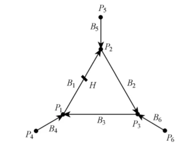
An artificial river network consists of cyclic looped channels based on real data was adopted in this study, as shown in Fig. 1.

The lengths of inside and outside channels were 10 km and 40 km, respectively. For the implicit discretization, the time step could be set from 5 to 60 min. Accounting for the simulation accuracy and computation burden, we used a 10-min time step in this study. The space interval was specified as 1 km.

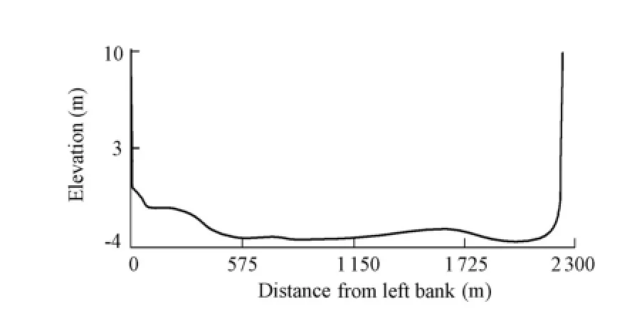
Three inner branches are marked as B1, B2, and B3, with the nodes P1, P2, and P3connecting with one another; three outer branches are marked as B4, B5, and B6, with the boundary nodes P4, P5, and P6assumed to be the Jiangyin, Yanglin, and Qinglonggang stations, respectively, near the Yangtze Estuary. The flow at the three gauge stations is significantly influenced by tides. In this study, the boundary conditions were specified with the observed water level from the Jiangyin, Yanglin, and Qinglonggang stations. The hydrological observation data of flood stage from 0:00 on June 28 to 0:00 on August 10, 1998 were selected for evaluating the efficiency of the water level updating model. The flow direction is presented with arrows in Fig. 1. If the computational result of a discharge is negative, the flow direction is opposite to the arrow direction. The transverse profile of the cross-section of the river channels is displayed in Fig. 2. In the river network, Manning’s roughness coefficient, mainly affecting the dynamic routing model, is about 0.02.

Fig. 1 Structure of artificial river network

Fig. 2 Profile of river channel cross-section

In this case, the high-resolution results of the dynamic routing model were taken as measurements in the updating scheme. For this purpose, the originally calculated situation should be changed to shorten the time step and space interval from 10 min and 1 km to 1 min and 50 m, respectively.

In order to test the efficiency of the updating model in forecasting the river network state without external interference, the middle cross-section H of B1was selected as themeasurement location (Fig. 1), and the calculated results of the water level updating model based on single water level correction values were compared with those obtained without adopting the water level updating model. The calculated results of the water level at inner nodes and discharge at cross-sections with and without adopting the water level updating model during the flood period from 2:00 on June 30 to 14:20 on July 16, 1998 are shown in Tables 1 and 2.

Table 1 Simulated results of water level at inner nodes with and without adopting updating model

Table 2 Simulated results of discharge at cross-sections with and without adopting updating model

From Tables 1 and 2, it can be seen that with water level updating, the values of RMSE of water level are less than 0.016 m, and those of discharge are less than 203.82 m3/s. The values of RMSE of water level with and without water level updating are almost the same at P3, the distance from which to the measurement point is larger than those from P1and P2. For the cross-sections SE2and SF3, the values of RMSE of discharge with water level updating are close to those without water level updating, and the largest value of RMSE (203.82 m3/s) occurs at SF3, indicating that the updating efficiency decreases with the increase of the distance from the cross-section to the measurement point.

In respect to the water level and discharge characteristics in the flood period, the results of the water level updating model with single water level correction values are much better than those without adopting the updating model. Thus, the water level updating model basedon single water level correction values is effective for water level and discharge forecasts.

3.2 Application to real river network

The Chengtong River network is located at the longitude from 120°15′E to 120°57′E and latitude from 31°45′N to 32°05′N from Jiangyin to Xuliujing. The model was applied to the Chengtong River network downstream of the Yangtze River, which consists of river channels with circular structures. Because the study area is beside the Yangtze Estuary, the water flow movement in this cyclic looped channel network is affected by both inflow from upstream and the tidal current from downstream. In the summer and fall seasons, the torrential rain falling in the river basin causes flood discharge over a 1- to 3-h period.

The four-point implicit finite difference approximation used in discretization of the dynamic wave equations is an unconditionally stable scheme. Hsu et al. (2006) demonstrated that the influences of the time step on dynamic routing are not significant. Accounting for the simulation accuracy and computation burden, we used a 15-min time step in this study.

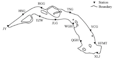
In the network, there are only three permanent water level stations, the Jiangyin (JY), Tianshenggang (TSG), and Xuliujing (XLJ) stations, providing a series of long-term observations. The other observation stations, including the Heshanggang (HSG), Rugaogang (RGG), Taiziwei (TZW), Jiulonggang (JLG), Wuganhe (WGH), Yingchuangang (YCG), Qiganhe (QGH), and Huifengmatou (HFMT) stations, shown in Fig. 3, are all temporary ones without long-term water level observations. The roughness coefficients in flood routing were classified into those of the main channel and flood plain by weight coefficients according to the real-time water level. The model was calibrated and verified with the measured water level from August 26, 2004 at 14:00 to September 18, 2004 at 11:50. The values of Manning’s roughness coefficient were calibrated against the observed flood events in August, 2004. The roughness coefficient of the main channel is around 0.025, and the value of the flood plain at both sides of the main channel is around 0.04. The upstream and downstream boundary conditions were specified based on the observed water level at the JY and XLJ stations, respectively.

Fig. 3 Distribution of observation stations along Chengtong River section

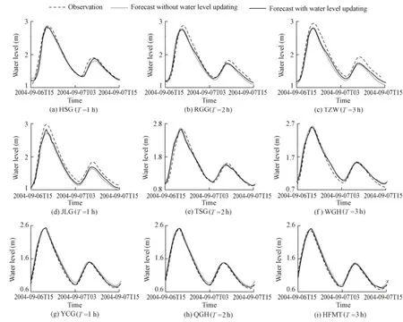
All measurement information from observation stations was incorporated into the water level updating model. Fig. 4 exhibits the forecasted hydrographs from 15:00 on September 6 to 15:00 on September 7, 2004, at nine observation stations based on 1- to 3-h flood routing using the water level updating model and the results of observation and obtained by the dynamic routing model. Fig. 4 reveals that the hydrographs of forecast results with water level updating are closer to those of observed data, showing a better prediction as compared with those obtained with the original dynamic routing model without water level updating, especially in a short lead-time forecast.

Fig. 4 Comparison of hydrographs at nine cross-sections obtained using water level updating model with a lead time from 1 to 3 h with those of observations and obtained by dynamic routing model

Detailed comparisons of the efficiency coefficients (E) and RMSE between the forecast results and observations at nine cross-sections for water level forecast with a lead time from 1 to 3 h are list in Table 3. Table 3 shows that the value of RMSE with water level updating increases with the lead time (T), while the value of E maintains a decreasing trend, demonstrating that the forecast accuracy of the water level updating model decreases with the increase of the lead time, and the effect of real-time updating gradually fades away with the increase of the forecast time.

Table 3 Model evaluation results of E and RMSE of water level forecast from September 6 to September 7, 2004

4 Conclusions

Based on the dynamic wave theory, a water level updating model was developed and applied in cyclic looped channel networks. With the discrete coefficients, the correction values obtained from observation stations can be extended from measurement points to other cross-sections nearby. The model was applied to ideal and real river networks, and some conclusions are as follows:

(1) The water level updating model shows a good performance in water level and discharge forecasts; its forecast accuracy is higher than the original dynamic routing model without water level updating, especially in a short lead-time forecast.

(2) The updating efficiency of the model in water level and discharge forecasts decreases with the increase of distance between the forecast position and the measurement point.

(3) Future research should be focused on systematic analysis of Manning’s roughness coefficient and its effect on flow forecasting.

Cheng, W. H., Wang, C. H., and Zhu, Y. 2006. Taihu Basin Model, 10, 71-77. Nanjing: Hohai University Press. (in Chinese)

Crissman, R. D., Chiu, C. L., Yu, W. Z., Mizumura, K., and Corbu, I. 1993. Uncertainties in flow modeling and forecasting for Niagara River. Journal of Hydrualic Engineering, 119(11), 1231-1250. [doi:10.1061/ (ASCE)0733-9429(1993)119:11(1231)].

Hsu, M. H., Fu, J. C., and Liu, W. C. 2003. Flood routing with real-time stage correction method for flash flood forecasting in the Tanshui River, Taiwan. Journal of Hydrology, 283(1-4), 267-280. [doi:10.1016/S0022-1694(03)00274-9]

Hsu, M. H., Fu, J. C., and Liu, W. C. 2006. Dynamic routing model with real-time roughness updating forflood forecasting. Journal of Hydraulic Engineering, 132(6), 605-619. [doi:10.1061/(ASCE) 0733-9429(2006)132:6(605)]

Kachroo, R. K. 1992. River flow forecasting, part 1: A discussion of the principles. Journal of Hydrology, 133(1-2), 1-15. [doi:10.1016/0022-1694(92)90146-M]

Kachroo, R. K., and Liang, G. C. 1992. River flow forecasting, part 2: Algebraic development of linear modelling techniques. Journal of Hydrology, 133(1-2), 17-40. [doi:10.1016/0022-1694(92)90147-N]

Lai, X. J. 2009. Real-updating multivariate analysis for unsteady flows with ensemble Kalman filter. Advances in Water Sciences, 20(2), 241-248. (in Chinese)

Li, Z. J., and Weng, M. H. 2001. Real-time flood forecasting modeling of 1D unsteady channel flow and kalman filter. Journal of Hydrodynamics, 13(1), 64-69.

Madsen, H., and Skotner, C. 2005. Adaptive state updating in real-time river flow forecasting: A combined filtering and error forecasting procedure. Journal of Hydrology, 308(1-4), 302-312. [doi:10.1016/ j.jhydrol.2004.10.030]

Mu, J. B., and Zhang, X. F. 2007. Real-time flood forecasting method with 1-D unsteady flow model. Journal of Hydrodynamics, 19(2), 150-154. [doi:10.1016/S1001-6058(07)60041-9]

Neal, J. C., Atkinson, P. M., and Hutton, C. W. 2007. Flood inundation model updating using an ensemble Kalman filter and spatially distributed measurements. Journal of Hydrology, 336(3-4), 401-415. [doi: 10.1016/j.jhydrol.2007.01.012]

Romanowicz, R. J., Young, P. C., and Beven, K. J. 2006. Data assimilation and adaptive forecasting of water levels in the river Severn catchment, United Kingdom. Water Resources Research, 42(6), 1-12. [doi:10.1029/2005WR004373]

Wang, C. H., and Bai, Y. L. 2008. Algorithm for real time correction of stream flow concentration based on Kalman filter. Journal of Hydrologic Engineering, 13(5), 290-296. [doi:10.1061/(ASCE)1084-0699 (2008)13:5(290)]

Wu, X. L., Xiang, X. H., Wang, C. H., Chen, X., Xu, C. Y., and Yu, Z. B. 2013. Coupled hydraulic and Kalman filter model for real-time correction of flood forecast in the Three Gorges interzone of Yangtze River, China. Journal of Hydrologic Engineering, 18(11), 1416-1425. [doi:10.1061/(ASCE)HE. 1943-5584. 0000473]

(Edited by Ye SHI)

——

This work was supported by the Major Program of the National Natural Science Foundation of China (Grant No. 51190091), the National Natural Science Foundation of China (Grant No. 51009045), and the Open Research Fund Program of the State Key Laboratory of Water Resources and Hydropower Engineering Science of Wuhan University (Grant No. 2012B094).

*Corresponding author (e-mail: freebird7237@163.com)

Received Jul. 15, 2012; accepted Dec. 7, 2012