Evaluation of 3D Time Domain Green Function Based on the Precise Integration Method

TONG Xiao-wang,REN Hui-long,LI Hui,SHAN Peng-hao

(College of Shipbuilding Engineering,Harbin Engineering University,Harbin 150001,China)

1 Introduction

It is an inevitable trend to analyze and solve the interaction problem between the wave and the structure in time domain.It will take up a lot of CPU storage space to establish and solve the integral equation in each time step,while using boundary element method to solve the hydrodynamic problem in time-domain.The key of this problem is how to calculate the time domain Green function quickly and accurately.Many researchers devoted themselves to the numerical computation of the time domain Green function and its derivatives,which are infinite range convolution integral with an oscillate kernel,and performance of highly frequency oscillation characteristics.According to oscillation properties of the integral type,Beck and Liapis(1987)[1]divided several computational domains,and using the series expansion or analytical formulation to solve time Green function.This method not only requires rich experience to determine computational domains and asymptotic expressions form,but also requires a large amount of computing time.Huang(1992)[2]proposed a Two Parametric interpolation technique which was adapted to the infinite depth of time domain Green function.This method improved the calculation efficiency while reduced the precision,and it does not apply to the calculation near the free surface.Based on the double parameter variables in bounded domain,Clement(1998)[3]and Shen Liang(2007)[4]presented a 4th ordinary differential equation(ODE)for three dimensional time domain Green Function in the infinite depth water.It will lead to numerical error after a long time when using Runge-Kutta method to calculate the time domain Green function ODE.

This paper obtains one kind of non-homogeneous and stationary system by modifying the time domain Green function ODE,which can be precisely solved by using the time PIM(Zhong Wanxie(1994)[5],Tan Shujun(2009)[6]).The method makes full use of the properties that time invariant systems are uniform about time.In other words,the motion equations remain the same properties about time.So,the time interval can be divided in to many tiny intervals,which makes the solution achieve to the analytical solution precisely and efficiently.

2 Time domain Green function and its ODEs

Consideration of the ideal fluid and flow irrotational,build the reference coordinate system as shown in Fig.1.The time domain Green function,which satisfies the free surface boundary conditions as referred in King(1987)[7],could be expressed as:

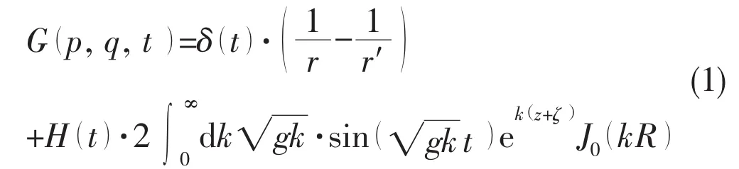
where δ（t）and H（t）are the Dirac impulse and the Heaviside step function,J0is the first kind of 0th order Bessel function.r and r′denote the distances between the source point p（x,y,z）and and field point q（ξ,η,ζ）,the source point and image of field point about still water,respectively.The first terms of G（p,q,t）in Eq.(1)is the impulsive partwhich can be simply calculated by using the Hess-Smith method.The second part of G（p,q,t）in Eq.(1)is termed as the memory part,which is the difficulty throughout the whole computation process.Now,the memory part denoted in the following paragraphs is the time domain Green function for the reason of describing expediently,as the form

with

From the Eq.(3),the main numerical calculation of the time domain Green functionis focusing on the double variables function F（μ,τ）,where（μ,τ）are two real variables,and 0≤μ≤1.

Clement(1998)pointed out that the form of double parameter function Av,l（μ,τ）,0≤μ≤1,defined as

is the solution of the ordinary differential equation

Compare to the Eq.(4)and Eq.(5),let v=0,l=1/2,F（μ,τ）satisfies the following fourthorder ordinary differential equation

By the same manner,we can obtain the horizontal derivative and the vertical derivative of

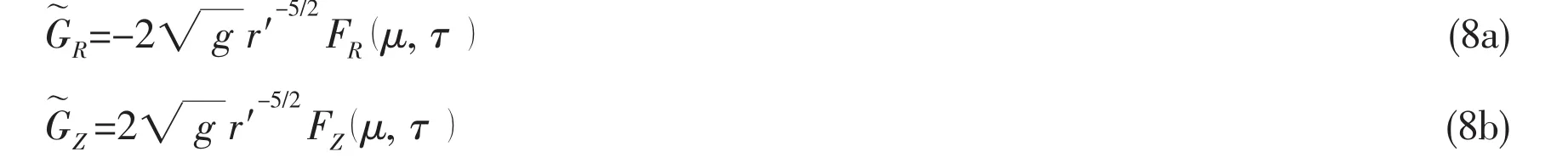
with

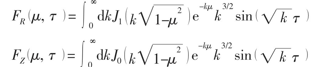
FR（μ,τ）andFZ（μ,τ）satisfy the following fourth-order ordinary differential equation,respectively

Suppose the base solution of Eq.(7)is:Eq.(7)can be reformed into the form

with

For the sake of brevity,the following paragraph omits the matrix’s subscript.

3 Numerical treatment

3.1 Introduction of Precise Integration Method

Reform the Eq.(10),the following new form can be obtained:

where A0is the linear stationary matrix,f（X,t）is nonlinear and non-homogeneous.For the practical problem of time domain Green function,define A0and f（X,t）forF（μ,τ）as

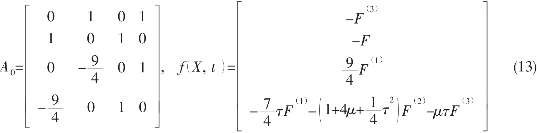
Obviously,the initial value of X（t）isthrough looking into theF（μ,τ）formulation.

The solution describing of Eq.(12),can be expressed with the Duhamel integral as

If suppose the dots of interval（tk,tk+1）as the initial time and the present time,so

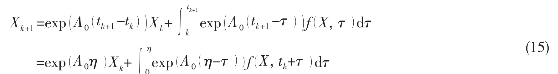
where,η=tk+1-tk,Xk≡X（tk）

Consider the intervals（tk-2,tk-1）and（tk-1,tk）,it will get the approximate Lagrange polynomialby using the linear explicit Adams method which contains the interpolate nodes tk-2,tk-1and tk

Introducing fk≡f（Xk,tk）,and take variable t+tkreplace t,Eq.(16)can be rewritten as

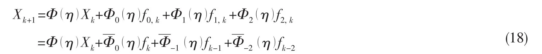
with

By looking into Eq.(18),the value at the present time tkneeds to determine previous values at tk-2,tk-1,tkand calculate the Duhamel integral precisely.In this paper,we employ the 4th Runge-Kutta method to confirm the 3 preceding time step values ofF（μ,τ）.

3.2 Precise integration of Duhamel integral

Divide the integral interval η into fine subsection,Commonly,when M is 20 there has 1 048 576 fine subsections,so the variable t is a super small magnitude.Therefore,Φ（η）can be expressed as the Taylor series expansion

The value k is confirmed by the order of an,k.For example of Φ2（t）,it needs to calculate an,kBecause the magnitude of variable t is very small,the Taylor series will truncated at 5th order,so Φ2（t）can be expressed as

Now,take care of the Duhamel integral property at time t=2t

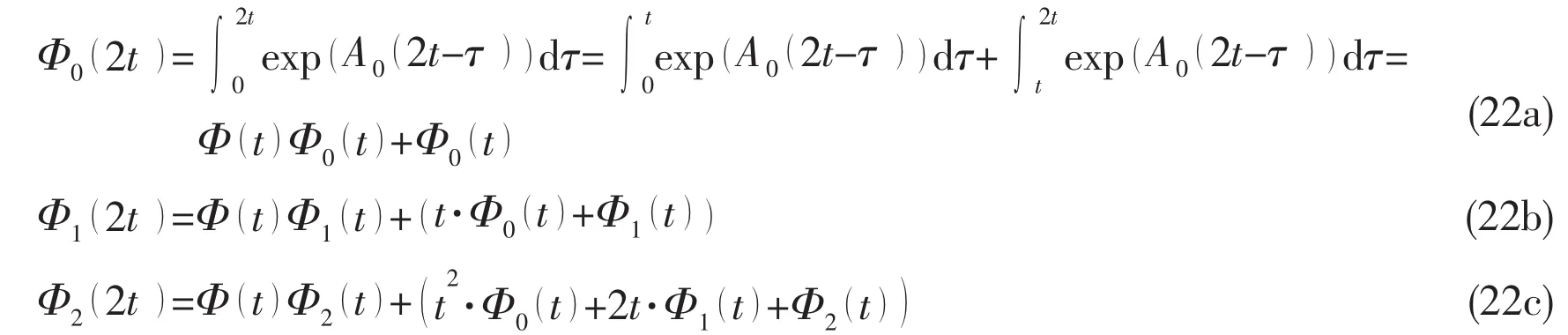
The magnitude of variable t is very small caused both Φ（t）and Φ（2t）approach to the unit matrix,so it must break out the increment part φ（t）and define φ（2t）is the increment at 2t.

Then it is time to study the relationship of Duhamel integralandover the entire interval η

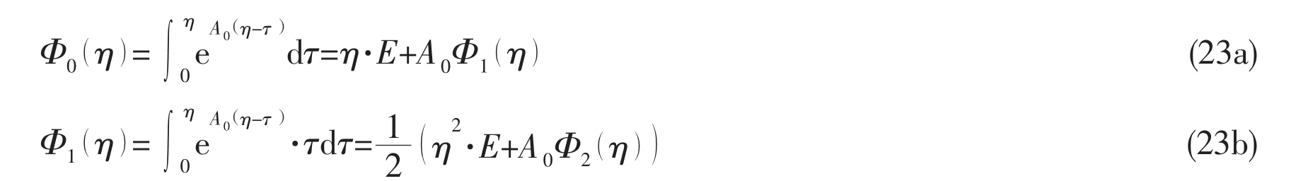
when obtained Φ2（η）,it is simply to confirmfrom Eq.(23b),and get Φ0（η）from Eq.(23a)further more.

4 Numerical results and analysis

F（μ,τ）and its derivatives,FR（μ,τ）,Fz（μ,τ）were computed by using PIM,at μ=0 and μ=1 for a range of τ.

In the case of μ=0,Clement(1998)afforded the analytic expression ofF（0,τ）

and pointed out that when τ→∞,F（0,τ）was always between the bounds of asymptotic lineand

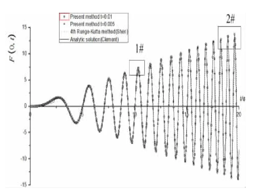
Fig.2 Comparison of F（0,τ）

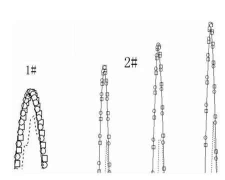
Fig.3 Zoom in F（0,τ）at 1#and 2#

The present method results were compared to those computed by Shen Liang(2007)and the analytic solution in Fig.2.It is easy to obtain the analytic solution by using the symbolic computation software Mathematica 6.0.In the work of Shen Liang,the 4th order Runge-Kutta Method was employed to compute the ODES of time domain Green function.For observing the difference among different methods carefully,the results in Fig.2 were locally zoomed in ofF（0,τ）at 1#and 2#as shown in Fig.3.Though the small time step is taken as 0.001,when calculated for a long time,the numerical accuracy declined after 10 s in the Shen Liang’s work.The algorithm damping of 4th order Runge-Kutta method is the main factor inducing the accuracy declined.The present method achieved the analytic solution perfectly when setting the bigger time step as 0.005 and 0.01.

In the other bound μ=1,Clement(1998)also afforded the analytic expression ofF（1,τ）

The M（x,y,t）function is called Hypergeometric Function M or Kummer’s function.The present results ofF（1,τ）were compared to analytic as shown in Fig.4.The curves in Figs.2-4,indicated that the present method has enough accuracy.The results ofF（μ,τ）about the double variables（μ,τ）were plotted in the Fig.5.It is easy to obtain the derivativesFR（μ,τ）andFZ（μ,τ）in the same process ofF（μ,τ）,whose results are plotted in Fig.6 and Fig.7,respectively.

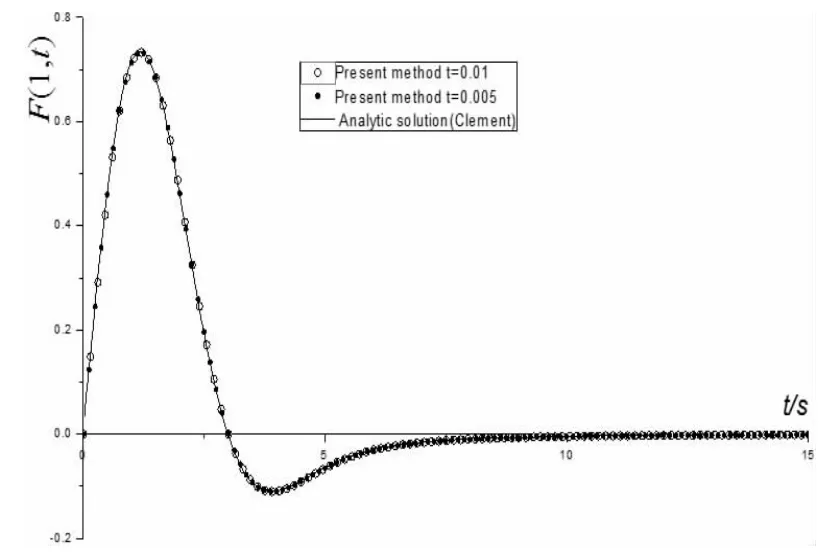
Fig.4 Comparison of F（1,τ）

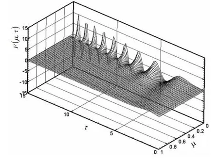
Fig.5 3D surface of F（μ,τ）

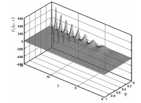
Fig.6 3D surface of FR（μ,τ）

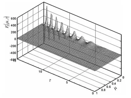
Fig.7 3D surface of FZ（μ,τ）

The 3D surface ofF（μ,τ）and its derivatives,FR（μ,τ）andFZ（μ,τ）are all consisting at 101×1 500 sets ofF（μ,τ）for 0≤μ≤1 and 0≤τ≤15.It takes about less than 5s on an Intel Core2 E7500(2.93GHz)PC,which indicated the present method is much more efficient than the former method.

5 Conclusions

It is the point to solve ship motions and responds in time domain that the efficient and accurate solution of time domain Green function and its derivatives.The method of 3D time domain Green Function and its derivatives in infinite depth was discussed in this paper.Based on the Precise Integration Method(PIM),the Green Function is obtained by solving a 4th order steady and non-homogeneous ordinary differential equations.Compared with the analytic and other methods,this method presented by this paper is achieving to exact solutions.It is accurate and efficient enough to solve the time domain Green function without high performance computers.

[1]Beck R F,Liapis S J.Transient motion of floating bodies at zero forward speed[J].Journal of Ship Research,1987,31(3):164-176.

[2]Huang Debo.Approximation of time-domain free surface function and its spatial derivatives[J].Ship Building,1992,4(1):16-25.

[3]Clement A H.An ordinary differential equation for Green function of time-domain free-surface hydrodynamics[J].Journal of Engineering Mathematics,1998,33(2):201-217.

[4]Shen Lian.A practical numerical method for deep water time-domain Green function[J].Journal of Hydrodynamics,Ser.A,2007,22(3):380-386.

[5]Zhong Wanxie.On precise time-integration method for structural dynamics[J].Journal of Dalian University of Technology,1994,34(2):131-136.

[6]Tan Shujun.Improvement of precise integration method and its application in dynamics and control[D].Ph.D.Thesis,Dalian University of Technology,Dalian,2009.

[7]King B K.Time-domain analysis of wave exciting forces on ship and bodies[D].Ph.D.Thesis,The University of Michigan,Ann Arbor,Michigan,1987.