Inter-textual Vocabulary Growth Patterns for Marine Engineering English

JINGJIE LI

(Donghua University, China)

ZHIWEI FENG

(The Ministry of Education; Dalian Maritime University, China)

1.INTRODUCTION

In 1957, J.R.Firth first put forward the theory of collocation, which separated the study of lexis from the traditional grammar and semantics.With the theory of collocation it became evident that the choice of vocabulary did not depend only on the grammatical structure.Neo-Firthians built on the lexis-oriented research approach and further developed Firth’s lexical theory.Halliday (1966: 148-162) presupposed the operation of lexis was at an independent linguistic level and was more than just filling in grammatical slots in a clause.

The vast amount of experimental studies and pedagogical publications has demonstrated, beyond all doubt, that the field of vocabulary studies is now anything but a neglected area (Schmitt 2002).The study of lexis has had a major influence on foreign language teaching, viz.as Smith (1999: 50) once commented on the significance of vocabulary, “the lexicon is of central importance and is even described as being potentially the locus of all variation between languages, so that apart from differences in the lexicon, there is only one human language.” Thus effective vocabulary acquisition is of particular importance for EFL learners (Ellis 2004) who frequently acquire impoverished lexicons despite years of formal study.

For effective vocabulary acquisition it is important that lexical items are acquired in certain quantities at certain rates.Thus, it is essential for both teachers and learners to be aware of the characteristics of vocabulary growth patterns such as vocabulary growth models and word frequency distributions.These characteristics are of practical significance not only for the resolution of a series of problems in vocabulary acquisition but also for the theoretical explanation of some of the important issues in quantitative lexical studies.

At present, quantitative lexical studies show characteristics of a multilayer development supported by computer technology and corpus evidence.Specifically, there have been many statistical approaches to the study of lexis acquisition.

Meara (1997) proposed a lexical uptake model (Equation 1.1) for incidental teaching and learning.A learner’s acquisition of vocabulary is expressed by a complex interaction between three variables: accumulated capacity of text input (N), number of new words provided in input texts (V(N)i), and likelihood of the learner picking up any individual word from those texts (p).

(1.1)

V(N): size of acquired vocabulary
V(N)i: the new vocabulary theithinput text provides
N: total number of input texts

pis an empirical parameter and its actual value is affected by teacher’s and learner’s experience, thus model 1.1 is factually determined by two factors, i.e.accumulated capacity of text input (N) and number of new words provided in input texts (V(N)i).These two factors constrain each other by some complex function relationship and define the vocabulary size of a learner.In other words, as long as we manage to simulate the function relationship ofNandV(N) (also called ‘vocabulary growth model’ in this paper), we can calculate the acquired vocabulary size and the vocabulary growth rate of a learner.In fact, many attempts have been made to construct an appropriate mathematical model that would express the dependence of the vocabulary sizeV(N) on the sample sizeN.Some models describe the vocabulary growth pattern for General English with sufficient precision, but none of them have ever been tested against the vocabulary development for Marine Engineering English (abbreviated henceforth as MEE).In this paper, four existing models (Brunet’s, Guiraud’s, Tuldava’s and Herdan’s models) will be tested against the empirical growth curve for MEE.Furthermore, a new growth model will be proposed and evaluated on the basis of Dalian Maritime University Marine Engineering English Corpus (abbreviated henceforth as DMMEE).

Some basic concepts and notation need to be delimited before making further analysis of vocabulary growth.To be consistent with the examination of current models, the vocabulary sizeV(N) in this paper is defined as the set of all lemmas in a given text, excluding Arabic numerals, non-word strings, and personal and place names, since the inclusion of these would gravely distort the vocabulary growth curves.However, the sizeNof a text or sample refers to the total number of any character cluster or a single character, including words, names, Arabic numerals, and non-word strings in the text, but excluding punctuation marks.

2.EXISTING VOCABULARY GROWTH MODELS

For much of the 20thcentury there has been a tradition of quantitative lexical studies with statistical information for various purposes.In the early 1930s, G.K.Zipf (1935) set out the rank-frequency law which held that the relationship between the frequency of the use of a word in a text and the rank order of that word in a frequency list is a constant.In the 1960s, Carroll (1967; 1969) put into words for the first time that word frequency distributions are characterized by large numbers of extremely low-probability words.This property sets quantitative lexical studies apart from most other studies in statistics and leads to particular statistical phenomena such as vocabulary growth patterns that systematically keep changing as the sample size is increased.In the 1980s and 1990s, special statistical techniques were developed to describe lexical frequency distributions accurately, and a number of vocabulary growth models were proposed.Of particular interest are Brunet’s, Guiraud’s, Tuldava’s, and Herdan’s models.

Expression 2.1 is known as Brunet’s model (1978), withlogwV(N) being the dependent variable andlogwNthe independent variable.

(2.1)

Hence,

W: Brunet’s constant serving as the base of the logarithmic function

ParameterWhas no probabilistic interpretation; it varies with the size of the sample.Parameterαis usually fixed at 0.17, a heuristic value that has been found to produce the desired result of producing a roughly constant relation betweenlogwV(N) andlogwN(Baayen 2001).

Expression 2.2 is known as Guiraud’s model (1990), where the square root of the sample size replaces the sample size in what is known as the type-token ratio,V(N)/N, as follows:

Hence,

(2.2)

R: Guiraud’s constant serving as the coefficient of the formula

The vocabulary sizeV(N) in Guiraud’s model reduces to a simple square function of the sample sizeN, but the parameterRchanges systematically with the sample size.

According to the hypothesis that the relation betweenV(N)/NandNis approximated by the power function:

Tuldava (1990) constructed a vocabulary growth model (Expression 2.3) by applying logarithmization to both variables ofV(N) andN.

(2.3)

e: natural base, e=2.17828...

Parametersαandβhave no probabilistic interpretation; they are the coefficients of variety that are supposed to be correlated with the probabilistic process of choosing “new” (unused) and “old” (already used in the text) words at each stage of text processing.

G.Herdan (1964) proposed a power model (Expression 2.4) based on the observation that the growth curve of the vocabulary appears as a roughly straight line in the double logarithmic plane.

(2.4)

αandβin Herdan’s model are empirical parameters; they have no sensible interpretation.

The current vocabulary growth models are of particular importance for the theory of quantitative statistics, but they are seldom used to solve practical lexico-statistical problems, either because their complex expressions are computationally rather intractable, or the model parameters keep changing systematically with the sample size.Moreover, thus far, none of the current growth models have been tested against the vocabulary development for MEE in the light of corpus evidence.

3.DMMEE AND METHODOLOGY

DMMEE was designed to represent the contemporary MEE; it consists of a little more than one million word tokens.Altogether 959 text samples were collected in the corpus; the length of each text varies from 349 to 2070 word tokens.Descriptive data of DMMEE are presented in Table 3.1.

Table 3.1 Detailed information on the size of DMMEE corpus

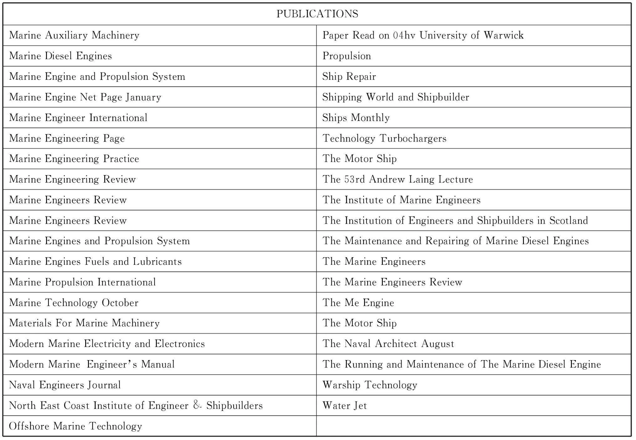
To achieve representativeness and balance in text sample selection, Summers (1991) outlined a number of possible approaches, including an “elitist” approach based on literary or academic merit or “influentialness”; random selection; “currency”; subjective judgment of “typicalness”; availability of text in archives; demographic sampling of reading habits; and empirical adjustment of text selection to meet linguistic specifications.By using a combination of theses approaches, 959 representative texts were selected from today’s most influential MEE materials that are produced or published in either Britain or the USA between 1987 and 2004.The titles of the publications are listed in Appendix A.

DMMEE is organized according to general genre categories such as papers and books.The quantity of text in each category complies roughly with the proportion of each material genre displayed in Appendix A.In DMMEE, about 85% of the text samples are taken from papers and books, 10% from lectures and discussions, and the remainder from such sources as brochures and manual instructions.Table 3.2 presents the general genre categories and their corresponding proportions.

Table 3.2 Overall structure and general genre categories of DMMEE corpus

The text samples of DMMEE were selected from various subject fields constituting MEE.Thus in the corpus one may find text samples on marine diesel engines, marine power plants, electrical installations, steering gears, marine refrigeration, gas exchange, lubricating systems, propelling systems, maintenance and repair, and so on.

3.切实发挥好四个作用。党员领导干部在市场开拓中要发挥好“管理协调”作用，在经营创收中要发挥好“引领激励”作用，在安全稳定中要发挥好“控制防范”作用，在精细管理中要发挥好“执行表率”作用。切实引导全体干部员工把思想汇聚到打造一流上、智慧集聚到打造一流上、力量凝聚到打造一流上，切实为公司发展挑重担、负责任，为员工当先锋、作表率。

With the aid of software SPSS and data-managing system FoxPro, and focussing on MEE vocabulary growth, this research aims:

A.To verify the descriptive power of current growth models from fitting the empirical growth curves of EST.

B.To construct a new growth model based on the analysis of current mathematical models.

C.To make a comparison of the new growth model with other known models in terms of parameter estimation, goodness of each model fit, and analysis of residuals.

D.To calculate the theoretical mean vocabulary sizes and their 95% two-sided tolerance intervals using the new model.

E.To plot the distributions of newly occurring vocabulary in cumulative texts.

Specifically, data processing was conducted in the following steps:

First, the text samples were randomly extracted from published texts in DMMEE and grouped into two sets, the Sample Set and the Test Set, each of which contained about 500,000 tokens.The Sample Set served as database for testing the four mathematical models and constructing a new vocabulary growth model.The Test Set was used to verify the descriptive power of the new model against MEE.

The number of text samples in each set is determined by two factors:

•The number of texts: the number of texts in the samples should be sufficiently large.Insufficient number of samples cannot capture true inter-textual lexical characteristics.In MEE, nearly 1000 texts (including Sample Set and Test Set) can basically capture true inter-textual lexical characteristics.

•The cumulative volume of texts: the total cumulative volume of texts in the samples should be large enough to produce sufficient vocabulary size of native speakers.Nation (1990) and Nagy (1997) place the vocabulary size of educated native speakers at 20,000.To be general, an EFL learner’s MEE vocabulary cannot be lower than that estimate.A test run revealed that cumulative texts of 500,000 word tokens can roughly cover the MEE vocabulary size of native speakers.(Fan 2006)

Information on the two sets is given in Table 3.3.

Table 3.3 Descriptive data for the Sample Set and the Test Set of DMMEE

The second step was to explore the newly occurring vocabulary distributions.The newly occurring vocabulary sizeV(N)newwas calculated and plotted as a function of the sample size N for both the Sample Set and the Test Set.Two respective FoxPro programs were designed to perform random selection of the text samples, and tokenization and lemmatization of each text sample.SPSS was used to plot the inter-textual vocabulary growth curves and the scatter-grams ofV(N)newagainst N for the two sets separately.

4.VOCABULARY GROWTH MODELS FOR MEE

To keep the integrity of the lexical structure of each individual text, the vocabulary growth curves plotted in this section are measured in units of text, not necessarily at equally spaced intervals.Figure 4.1 plots the dependence of the vocabulary sizeV(N) on the sample sizeNfor the Sample Set and the Test Set of DMMEE.

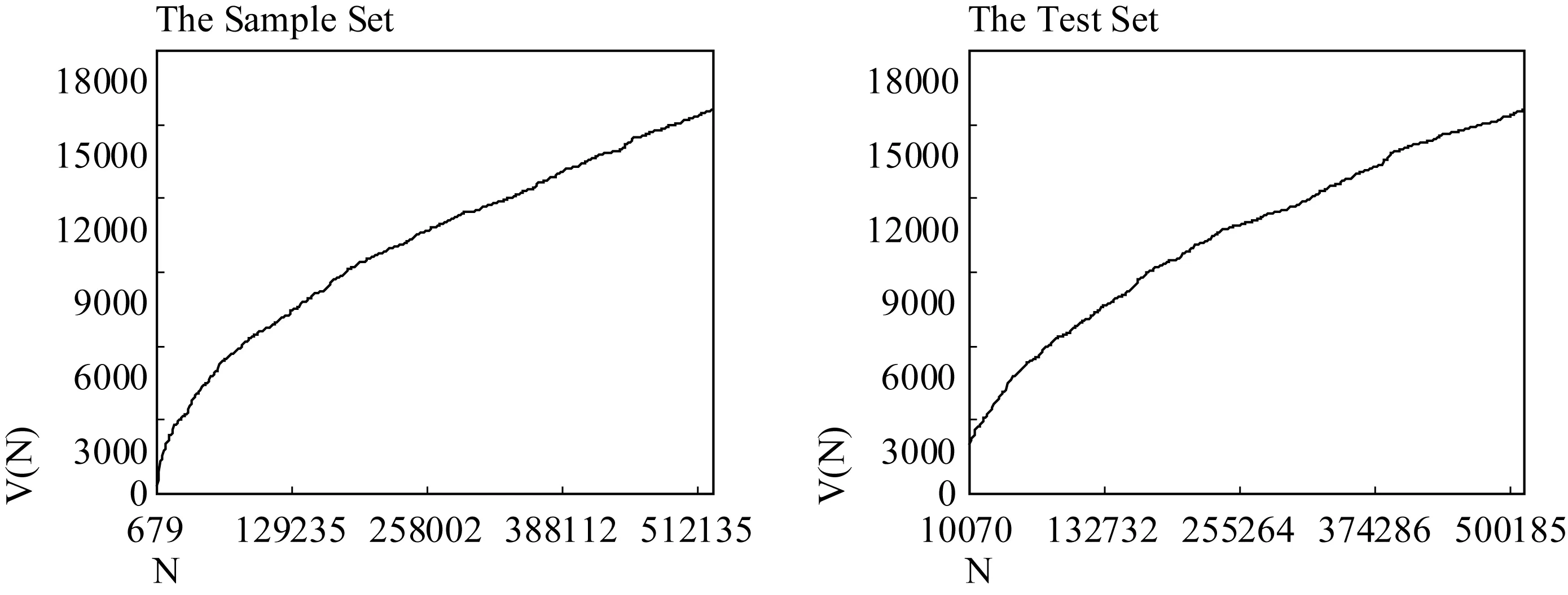
Figure 4.1 Vocabulary size V(N) as a function of sample size N for the cumulative texts in the Sample Set (left panel) and the Test Set (right panel) of DMMEE.

The vocabulary growth curves for the Sample Set and the Test Set exhibit similar patterns.For example, the growth curve ofV(N) in the left panel is not a linear function ofN.Initially,V(N) increases quickly, but the growth rate decreases as N is increased.By the end of the Sample Set the curve has not flattened out to a horizontal line, that is, the vocabulary size keeps increasing even when the sample size has reached 500,000 word tokens.

4.1 Test of the Existing Vocabulary Growth Models

Figure 4.2 plots the empirical vocabulary growth curve (tiny circles) for the Sample Set, as well as the corresponding expectations (solid line) using Brunet’s, Guiraud’s, Tuldava’s and Herdan’s models.

Brunet’s model (upper left panel) fits the empirical growth curve well.The value of R square (the coefficient of determination) reaches 99.876%.However, the upper left panel shows that Brunet’s model underestimates the observed vocabulary sizes both at the beginning and towards the end of the growth curve.The predicted values are presented in the third column of Appendix B (Pred_B).

Guiraud’s model (upper right panel) does not fit the empirical growth curve quite well.The R square is 99.812%, the lowest value among the four models.The upper right panel shows that Guiraud’s model overestimates the observed vocabulary sizes from the beginning of the growth curve to nearly the middle.The predicted values are listed in the fifth column of Appendix B (Pred_G).

The fit of Tuldava’s model (lower left panel) is close to the empirical growth curve, with theRsquare reaching 99.910%.But Tuldava’s model tends to underestimate the observed vocabulary sizes at the beginning of the curve.The expected values are presented in the seventh column of Appendix B (Pred_T).

Though similar in expression to Guiraud’s model, Herdan’s model (lower right panel) describes the empirical growth curve best of the four models.TheRsquare reaches the highest value 99.942%.But the panel shows that Herdan’s model tends to overestimate the observed vocabulary sizes towards the end of the growth curve.The expected values are listed in the ninth column of Appendix B (Pred_H).

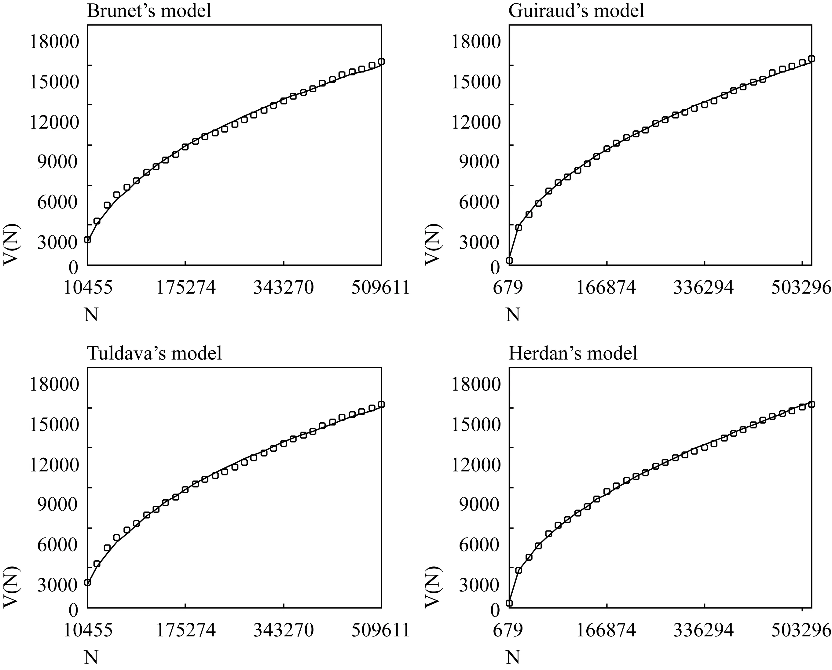
Figure 4.2 Observed (tiny circles) and expected (solid line) vocabulary growth curves for the Sample Set.The upper left panel shows the fit of Brunet’s model to the empirical values, the upper right panel the fit of Guiraud’s model, the lower left panel the fit of Tuldava’s model, and the lower right panel the fit of Herdan’s model.

4.2 A New Vocabulary Growth Model for MEE

Based on the lexico-statistical study of the Sample Set, a new mathematical model (Expression 4.1) is suggested to fit the vocabulary growth curve for MEE.

(4.1)

The new model is constructed by multiplying the logarithmic function and the power law.Parameterαis the coefficient of the whole expression; parameterβis the exponential of the power function part of the model.Parametersαandβdo not have fixed values; they have to change slightly with specific sample sizes to realize sufficient goodness-of-fit.

The theoretical considerations for proposing the new model are as follows:

•Brunet’s model is in essence a complex logarithmic function, with logWNbeing the independent variable and logWV(N) the dependent variable.It tends tounderestimatethe observed vocabulary sizes both at the beginning and towards the end of the empirical growth curve.

•Herdan’s model is a generalized power function.It tends tooverestimatethe observed values towards the end of the vocabulary growth curve.

•The mathematical combination of the logarithmic function and the power law may provide good fit to the empirical growth curve for MEE.

Figure 4.3 plots the dependence ofV(N) on N for the Sample Set and the expectations using the new growth model.

The new mathematical model provides very good fit to the empirical growth curve.The value ofRsquare reaches 99.945%, higher than any other vocabulary growth models, particularly Brunet’s model and Herdan’s model.The respective values of parametersαandβare 3.529696 and 0.442790 for the Sample Set.

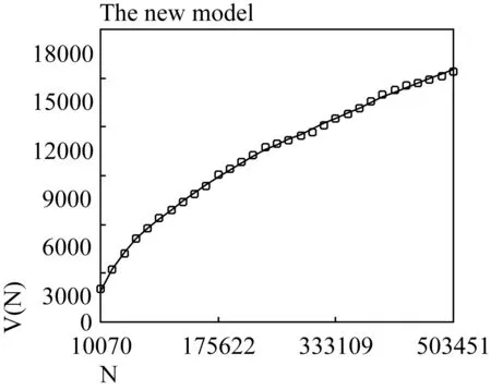
Figure 4.3 Vocabulary size V(N) as a function of the sample size N, measured in units of text.The tiny circles represent the empirical growth curve for the Sample Set, and the solid line the expected growth curve derived from the new mathematical model.

4.3 Goodness-of-Fit Test for the New Vocabulary Growth Model

The Test Set of DMMEE is used to evaluate the descriptive power of the new vocabulary growth model.Figure 4.4 plots the empirical growth curve for the Test Set (tiny circles) and the corresponding expectations using the new mathematical model (solid line), withα=3.529696 andβ=0.442790.

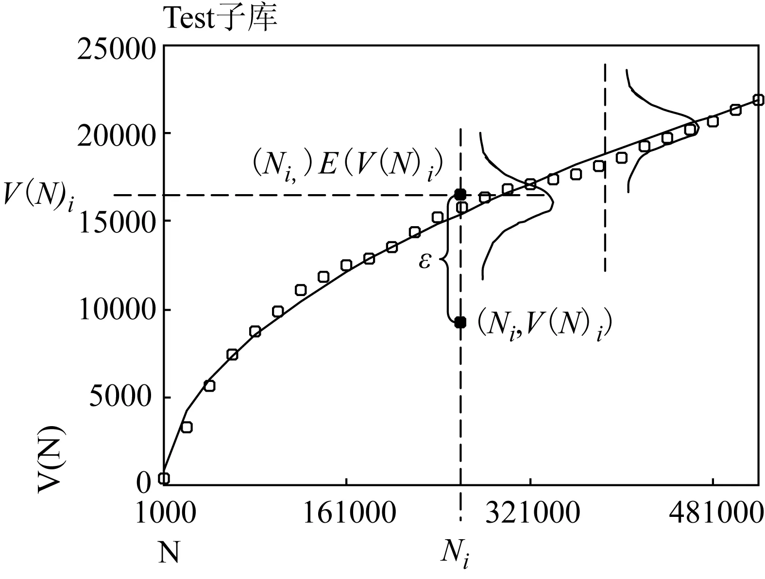
Figure 4.4 Dependence of the vocabulary size V(N) on the sample size N, measured in units of text.The tiny circles represent the empirical growth curve for the Test Set, and the solid line represents the expected growth curve derived from the new mathematical model.

The Sample Set has similar corpus size with the Test Set, and they both represent the contemporary MEE.Thus, the observed values of parametersαandβderived from the Sample Set also apply to the Test Set.Figure 4.4 shows that the new model provides good fit to the growth curve for the Test Set.The value of R square reaches 99.917%.

The new growth model is probabilistic in nature, so the appropriate generalization to this new model assumes that the expected value ofV(N) is the function ofN, but the variableV(N)idiffers from its expected value in a random deviationε(Expression 4.2).

(4.2)

The standard deviation ‘s’ determines the extent to which each normal curve of vocabulary spreads out about its mean value E(V(N)i).(Figure 4.4) When ‘s’ is small, the observed point (Ni,V(N)i) probably falls quite close to the theoretical growth curve; whereas observations may deviate considerably from their expected vocabulary sizes when ‘s’ is large (Devore 2000).In order to calculate the standard deviation value for each point (N,V(N)) in units of text, the text samples of DMMEE are randomly selected and rearranged into ten sets of samples, based on which ten sets of vocabulary sizes and their corresponding sample sizes are obtained and displayed in Appendix C.Devore proposed that whennsample=10 (number of samples), the tolerance critical value is 3.379 for capturing at least 95% of the observed values in the normal population distribution.

SPSS calculates the two-sided tolerance interval for each point (Ni,V(N)i) on the expected growth curve with a confidence level of 95%.Table 4.1 displays part of the statistics, including the standard deviationsand the corresponding upper and lower bound vocabulary sizes.

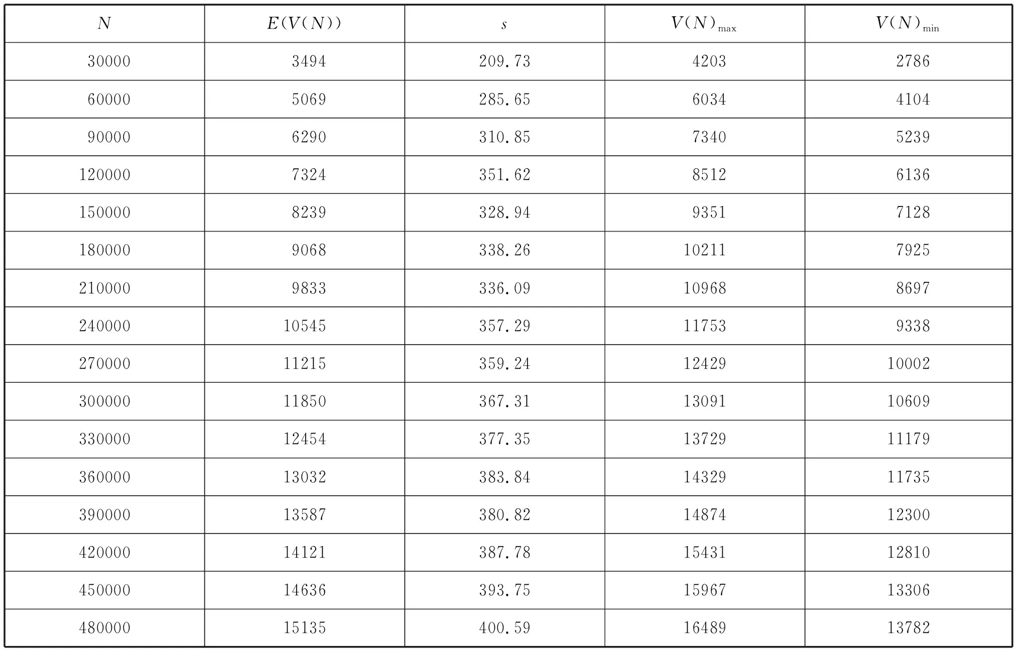
Table 4.1 Sample size N, theoretical vocabulary mean E(V(N)), standard deviation ‘s’,upper bound vocabulary size V(N)max and lower bound vocabulary size V(N)min for each point (N, V(N)) on the expected growth curve derived from the new model

Figure 4.5 plots the empirical growth curve for the Test Set and the upper and lower bound values using the new mathematical model.The dashed lines show that the observed vocabulary sizes fall within the 95% two-sided tolerance bounds, without any exceptions.

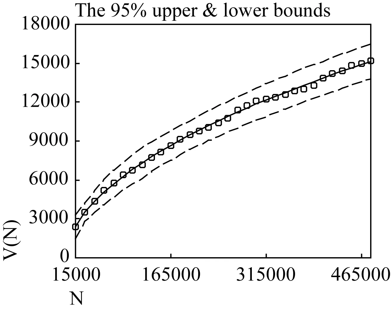
Figure 4.5 V(N) as functions of N, measured in units of text. The tiny circles represent the empirical growth curve for the Test Set, the solid line the theoretical expectations using the new model, and the dashed lines the upper and lower bound curves for a confidence level of 95%.

4.4 Analysis of Residuals for Vocabulary Growth Models

Vocabulary sizes that did not fit the empirical growth curve, hereafter residuals-from-fit, will be analysed for their variance and the degree to which there are coherent patterns in the residuals.

The variance of residuals shows how accurately the growth models predict the vocabulary values.A smaller variance implies a better fit of the model to the empirical growth curve and lower statistical uncertainty of the model components.SPSS calculates the mean square (a measure of variance) of residuals-from-fit for each vocabulary growth model.(Table 4.2)

Table 4.2 Mean square values (variance) of residuals-from-fit for each of the five vocabulary growth models in the Test Set

The new mathematical model fits the empirical growth curve best, with the mean square value of residuals being the lowest.Herdan’s model, Tuldava’s model, Brunet’s model and Guiraud’s model follow in a sequence of decreasing goodness-of-fit.

In view of Scheaffer (1973), if the model makes correct predictions of the observed values, there should be no coherent patterns in the distribution of residuals.The greater the coherent structure of the residuals, the greater the chance that the observations deviate from their expected values.Figure 4.6 shows the residual plot against the sample size of the five vocabulary growth models.

The residuals from the new model exhibit no coherent patterns (solid line).The residuals are randomly distributed about their expected values 0 (dashed line) according to a normal distribution.All but a very few residuals lie between -160 and 160.

The residuals from the other four growth models (dotted lines) exhibit coherent patterns, such as a curved pattern for Brunet’s model and an increasing function for Guiraud’s model.The respective residuals fall within the interval of [-223, 397] for Brunet’s model, [-305, 299] for Guiraud’s model, [-209, 300] for Tuldava’s model, and [-150, 220] for Herdan’s model.

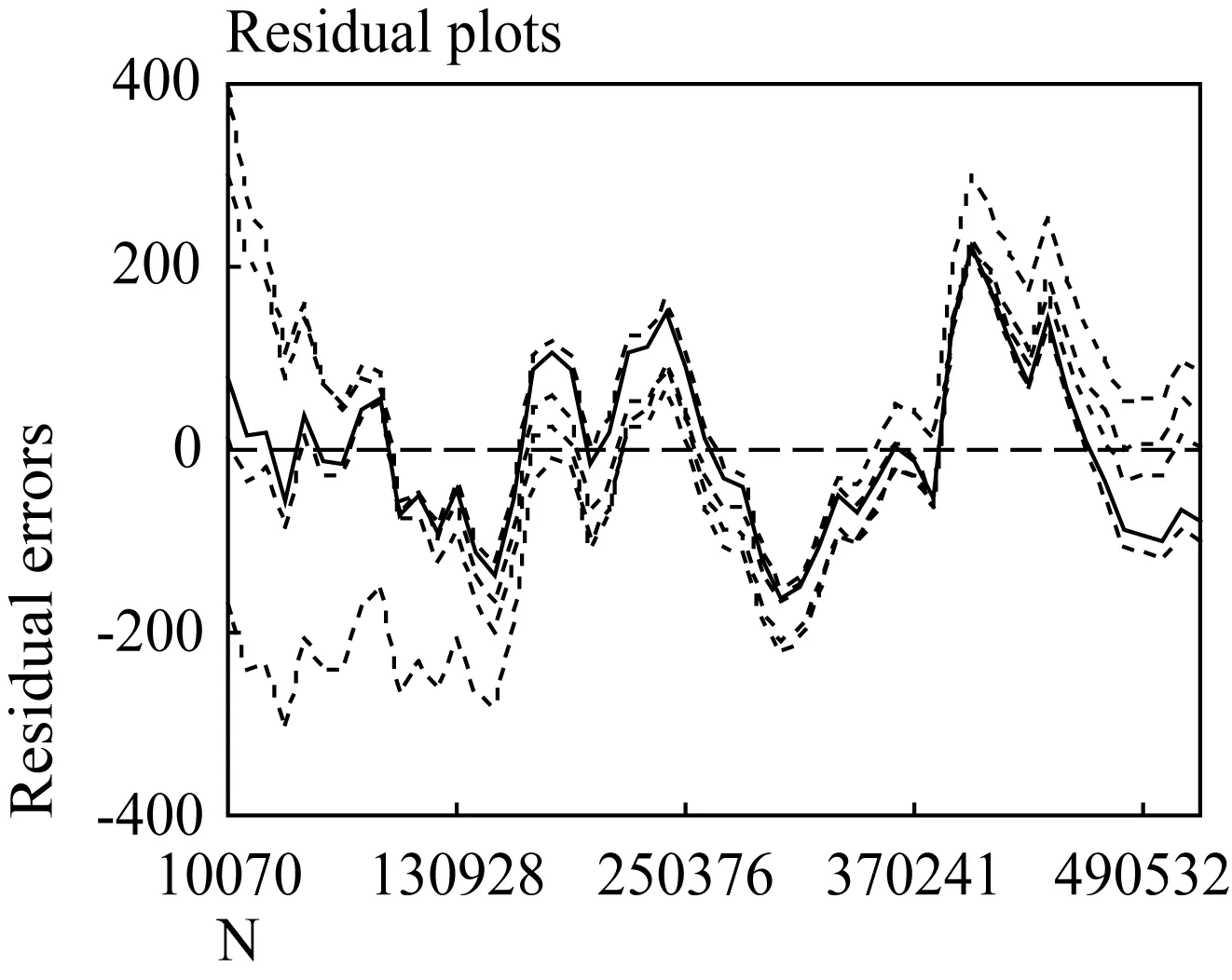
Figure 4.6 Residuals as functions of the sample size N, measured in units of text.The solid line represents the residuals from the new model, the dotted lines the residuals from the other four growth models, and the dashed line the expected value for each residual error.

The new model accounts for the empirical growth curve best of the five models for both the Sample Set and the Test Set.Therefore, it is reasonable to conclude that the new model gives the most accurate predictions of vocabulary growth for MEE.Tables 4.3 and 4.4 present the detailed information and basic statistics for the goodness of each model fit.

Table 4.3 Expressions and parameters of the vocabulary growth models for the Sample Set and the Test Set

Table 4.4 Goodness-of-fit statistics (R square and mean square values) for the five models from fitting the empirical growth curves for the Sample Set and the Test Set

5.NEWLY OCCURRING VOCABULARY DISTRIBUTIONS IN CUMULATIVE TEXTS

Feng (1988, 1996) proposed the “law of decreasing new vocabulary growth” in his study of terminology.He noticed that with the increase of terminology entries, the number of high frequency words grows correspondently, whereas the probability of the occurrence of new words decreases.At this point, although the number of terminology entries keeps growing, the growth rate of the total number of new words slows down.The repeated occurrences of high frequency words indicate a tendency of decreasing new vocabulary growth.“The law of decreasing new vocabulary growth” lends itself not only to terminology system but also the process of reading written texts.When starting to read a text written in a less familiar language, one may encounter a body of new words.As more texts are read, the growth rate of new words is gradually reduced.If the reader can master the new words he comes across, reading will be much easier.There exists a function relationship between the number of new words (W) and text capacity (T) as follows:

With the increase of text capacity (T), the growth rate of the number of new words (W) begins to reduce and the function curve becomes smoother in a form of convex parabola in the rectangular coordinate system.This function curve indicates the process of vocabulary growth in the reading of written texts.It is a mathematical account of the law of vocabulary change in a reading process.

The corpus evidence proves Feng’s theory and suggests that as the sample sizeNincreases, the new vocabularyV(N)newthat an additional input text produces decreases.At any givenNithe new vocabularyV(N)newof a sample with N word tokens can be estimated with Expression 5.1.

(5.1)

Figure 5.1 plots the newly occurring vocabulary sizeV(N)newas a function of the sample sizeNfor the Sample Set and the Test Set.

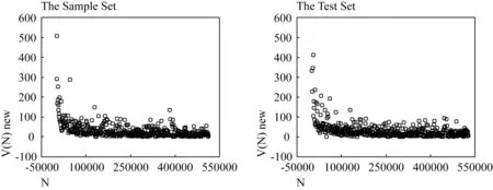
Figure 5.1 Scatter-grams of V(N)new against N for the Sample Set (left panel) and the Test Set (right panel)

The left panel for the Sample Set and the right panel for the Test Set reveal surprisingly similar distributions of newly occurring vocabulary sizes.The new vocabularyV(N)newis a rapidly decreasing function of the sample size N with a long tail of the low values ofV(N)new.Initially,V(N)newdecreases sharply to some steady-state value that decreases slowly and smoothly.Then as N increases, the empirical values ofV(N)neware distributed about the stable value in a wide dispersion till the end of the scatter plot.Take the left panel into consideration; the first input text produces more than 500 new word types.ThenV(N)newdecreases sharply asNincreases, viz.when the sample size reaches 62,305 word tokens, the value ofV(N)newis reduced to less than 150.But fromN=62,305 onwards till the end of the scatter plot, the newly occurring vocabulary size decreases very slowly and the observed values ofV(N)neware distributed in a fluctuant way.The last input text produces 6 new word types, which proves that new vocabulary still occurs even when the sample size has reached 500,000 word tokens.

6.EXAMPLES OF PEDAGOGICAL APPLICATIONS

This research has significance in explicit EFL teaching and learning.With the assistance of the new growth model, teachers and students can make reliable estimates not only on the vocabulary size and its intervals for a given textbook but also on the volume of texts that are needed to produce a particular vocabulary size.For example, suppose that a textbook of MEE consists of 50 input texts, with the size of each text varying between 500 and 2,000, and totalling 50,000 word tokens.The vocabulary size of the whole textbook is estimated by using the new growth model, withα=3.5297 andβ=0.4428:

The 95% tolerance interval is calculated to estimate the possible vocabulary sizes, withcriticalvalue=3.379 ands=118.1479:

Thus we are “95% certain” that the vocabulary size of the whole textbook lies between 4199 and 4998 word types.If 5% of the total vocabulary input fails to be acquired, then the two-sided tolerance interval for the acquired vocabulary is [4199-4199×5%, 4998-4998×5%], that is, [3989, 4748].If a new text with 1000 tokens is added into the textbook, the newly occurring types that this input text produces are estimated according to Expression 5.1:

The 95% tolerance interval is calculated for the newly occurring vocabulary, withcriticalvalue=3.379 ands=10.1751:

Another example is to estimate the sample size for a given vocabulary size.For example, The Engineering English Competence Examination has a fairly high requirement on vocabulary proficiency with the minimal limit of 4000 word types.To ensure sufficient amount of vocabulary, the textbook of MEE has to reach a certain size.According to the new growth model, the expected size of the textbook is calculated as follows:

With criticalvalue=3.379 ands=2231.342, the 95% tolerance interval is:

Thus we are at least “95% confident” that the size of the textbook of MEE has to be between 31010 and 46090 tokens, in order to produce 4,000 word types.

7.CONCLUSION

This paper explores two fundamental issues concerning the inter-textual vocabulary growth patterns for MEE: the vocabulary growth models and newly occurring vocabulary distributions in cumulative texts.

The paper first explores the MEE vocabulary growth.The growth curve of vocabularyV(N) is not a linear function of the sample sizeN.Initially,V(N) increases quickly, but the growth rate decreases asNis increased.Four mathematical models (Brunet’s, Guiraud’s, Tuldava’s and Herdan’s models) are tested against the empirical growth curve for MEE.A new growth model is constructed by multiplying the logarithmic function and the power law.Parameterαis the coefficient of the whole expression; parameterβis the exponential of the power function part of the model.

The new model describes the empirical growth curve best of the five models for MEE, with theRsquare reaching the highest value and the mean square being the lowest.The upper and lower tolerance bounds are calculated to capture at least 95% of the possible vocabulary sizes in the normal population distribution.The residuals from the five growth models are compared and analyzed; the respective values fall within the interval of [-223, 397] for Brunet’s model, [-305, 299] for Guiraud’s model, [-209, 300] for Tuldava’s model, [-150, 220] for Herdan’s model, and [-160,160] for the new model.

The second issue this paper explores is the distribution of newly occurring vocabulary sizes in cumulative texts.The new vocabularyV(N)newis a rapidly decreasing function of the sample sizeNwith a long tail of low values ofV(N)new.Initially,V(N)newdecreases sharply to a certain point.Then asNincreases,V(N)newdecreases very slowly and its observed values are distributed in a fairly wide dispersion.

The present study has been exploratory in nature, and some difficult issues have not yet been tackled adequately.For example, the new vocabulary growth model was constructed on the basis of studies of the Sample Set, which consists of 480 individual texts, totalling about 500,000 word tokens.The model has been verified to provide good fit to the empirical vocabulary sizes within the boundary of the sample size of not more than 500,000 word tokens.However, the possibilities of extrapolation of this new growth model in the direction of larger than 500,000 tokens need further consideration and verification.

REFERENCES

Baayen,R.H.2001.WordFrequencyDistributions.Dordrecht: Kluwer Academic Publishers.

Brunet,E.1978.LeVocabulairedeJeanGiraudoux.Geneve：SLATKINE.

Carroll,J.B.1967.ComputationalAnalysisofPresent-DayAmericanEnglish.Providence: Brown University Press.

Carroll,J.B.1969.ARationaleforanAsymptoticLognormalFormofWordFrequencyDistributions.Princeton: Research Bulletin, Educational Testing Service.

Devore,J.2000.ProbabilityandStatistics.Pacific Grove: Brooks/Cole.

Ellis,R.2004.SecondLanguageAcquisition(5thedition).Shanghai: Foreign Language Teaching Press.

Fan,Fengxiang.2006.‘A corpus-based empirical study on inter-textual vocabulary growth,’JournalofQuantitativeLinguistics13/1: 111-127.

Feng,Zhiwei.1988.‘FEL formula—Economical law in the formation of terms,’ Information science 9/5: 8-15, 96.

Feng,Zhiwei.1996.IntroductionofModernTerminology.Beijing: The Language Publishing House.

Feng,Zhiwei.2006.‘Evolution and present situation of corpus research in China,’InternationalJournalofCorpusLinguistics11: 173-207.

Guiraud,H.1990.LesCaracteresStatistiquesduVocabulaire.Paris: Presses Universitaires de France.

Herdan,G.1964.QuantititativeLinguistics.London: Buttersworths.

Kennedy,G.2000.AnIntroductiontoCorpusLinguistics.Beijing: Foreign Language Teaching and Research Press.

Schmitt,N.andP.Meara.1997.‘Researching vocabulary through a word knowledge framework: Word associations and verbal suffixes,’StudiesinSecondLanguageAcquisition19: 17-36.

Schmitt,N.andM.McCarthy.2002.Vocabulary:Description,AcquisitionandPedagogy.Shanghai: Shanghai Foreign Language Education Press.

Sinclair,J.1991.Corpus,Concordance,Collocation.Oxford: Oxford University Press.

Smith,N.1999.Chomsky:IdeasandIdeals.Cambridge: Cambridge University Press

Summers,D.1991.Longman/LancasterEnglishLanguageCorpus:CriteriaandDesign.Harlow: Longman.

Tuldava,J.1996.‘The frequency spectrum of text and vocabulary,’JournalofQuantitativeLinguistics3: 38-50.

Zipf,G.K.1935.ThePsycho-BiologyofLanguage.Boston: Houghton Mifflin.

Zipf,G.K.1949.AnIntroductiontoHumanEcology.New York: Hafner.

Appendix A

The titles of the publications from which text samples were selected for DMMEE

(Continue)

Appendix B

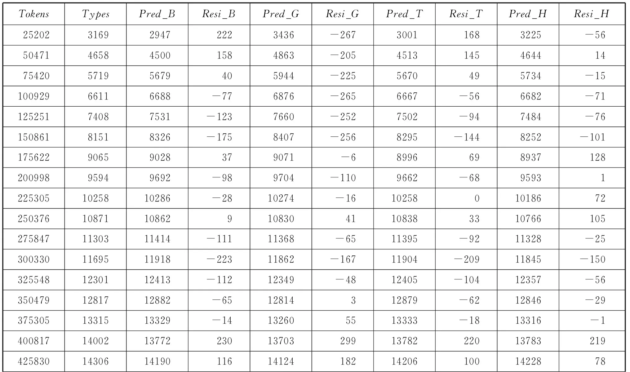
Part of Statistics for the Sample Set Using Brunet’s Model, Guiraud’s Model, Tuldava’s Model and Herdan’s Model

(Continue)

Appendix C

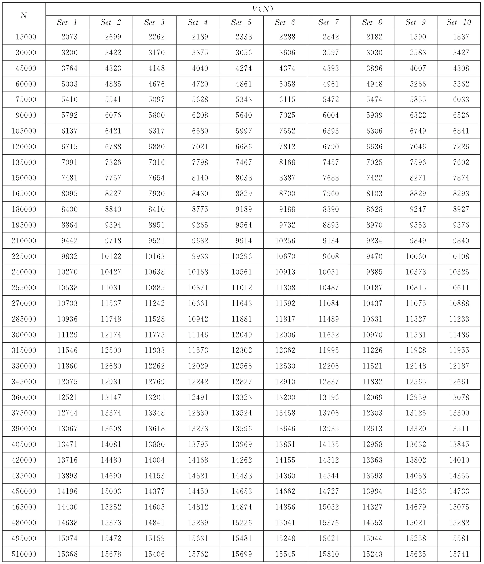
Statistical Data for the Ten Sets of Text Samples